How To Hide Data with Checkboxes in Google Sheets

Welcome To Better Sheets!

Let's explore the magical the magical things you can do with checkboxes in Google Sheets.

This may be the most underused feature in Google Sheets but this adds a mighty functionality to your sheets. That is combining Checkboxes with Formulas.

It turns out to be like a magic trick.

Let's begin and make the most out of it.

1. Inserting Checkboxes

Adding Checkboxes in Google Sheets is very simple.

• Navigate Insert Tab and select "Tick box" (this used to be Checkbox)

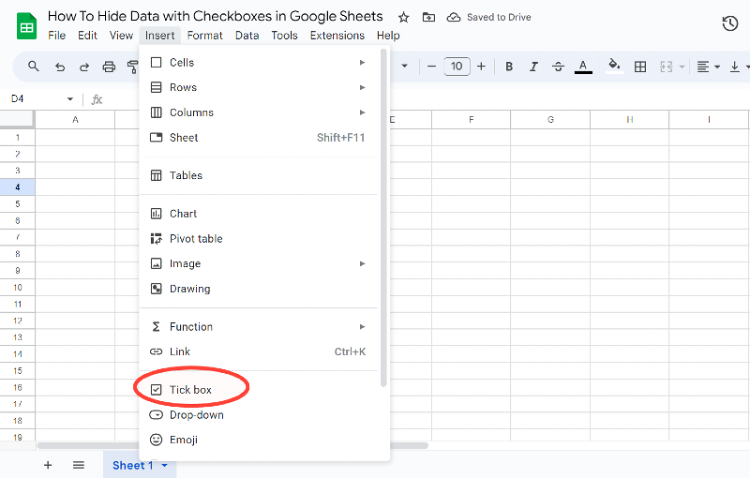
As simple as that and you're all set. You have a checkbox or tick box that you can switch between True or False.

2. Getting Started with Checkboxes

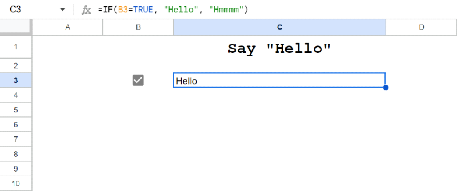
Let's start with the basic and fun use of checkboxes. Let's say you want your check box to say "Hello" when checked and "Hmmm" when unchecked. This is we're gonna do it.

• Insert a Checkbox. Click on the cell where you want your checkbox to be placed.
• Apply a Formula: Use the formula:

=IF(B3=TRUE, "Hello", "Hmmmm")

This formula will check if the box in cell B3 is true (checked) and cell C3 displays "Hello."

If unchecked, it shows "Hmmm."

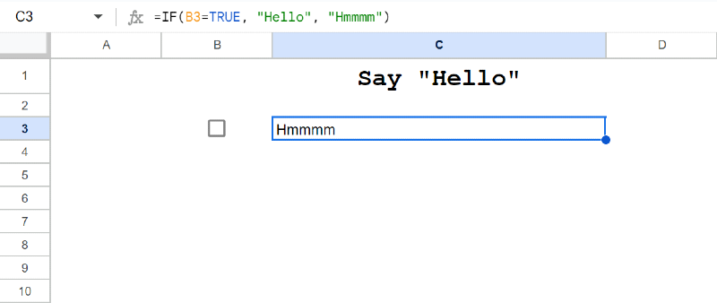
This is just a fun and simple example, but it shows the potential of combining checkboxes with formulas to create dynamic content.

3. Hiding Data with Checkboxes

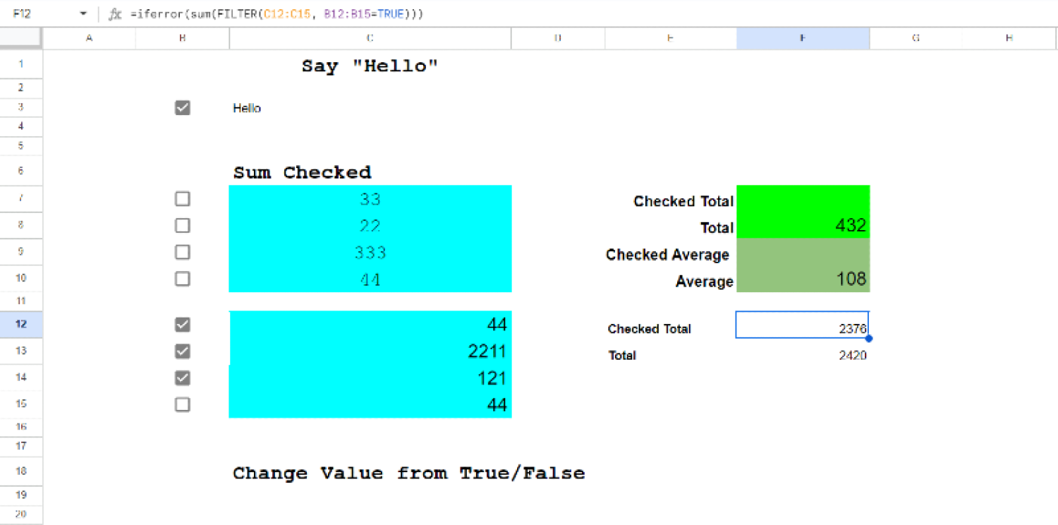
One of the most powerful uses of checkboxes is to hide or show data. Let’s say you have a range of numbers and you want to know the sum of the only ones you've checked. Checkboxes make this possible and incredibly easy.

• Insert Checkboxes. Place checkboxes next to the numbers you want to include in your sum.
• Add the Numbers. Enter your numbers in cells. For example, C7:C15.

Sum Checked Values. Use the formula:

=IFERROR(SUM(FILTER(C12:C15, B12:B15=TRUE)))

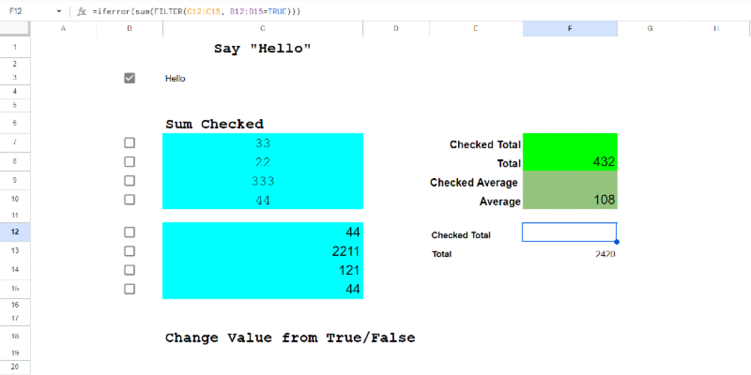
This sums the values in range C12only if the corresponding checkbox in B12is checked.

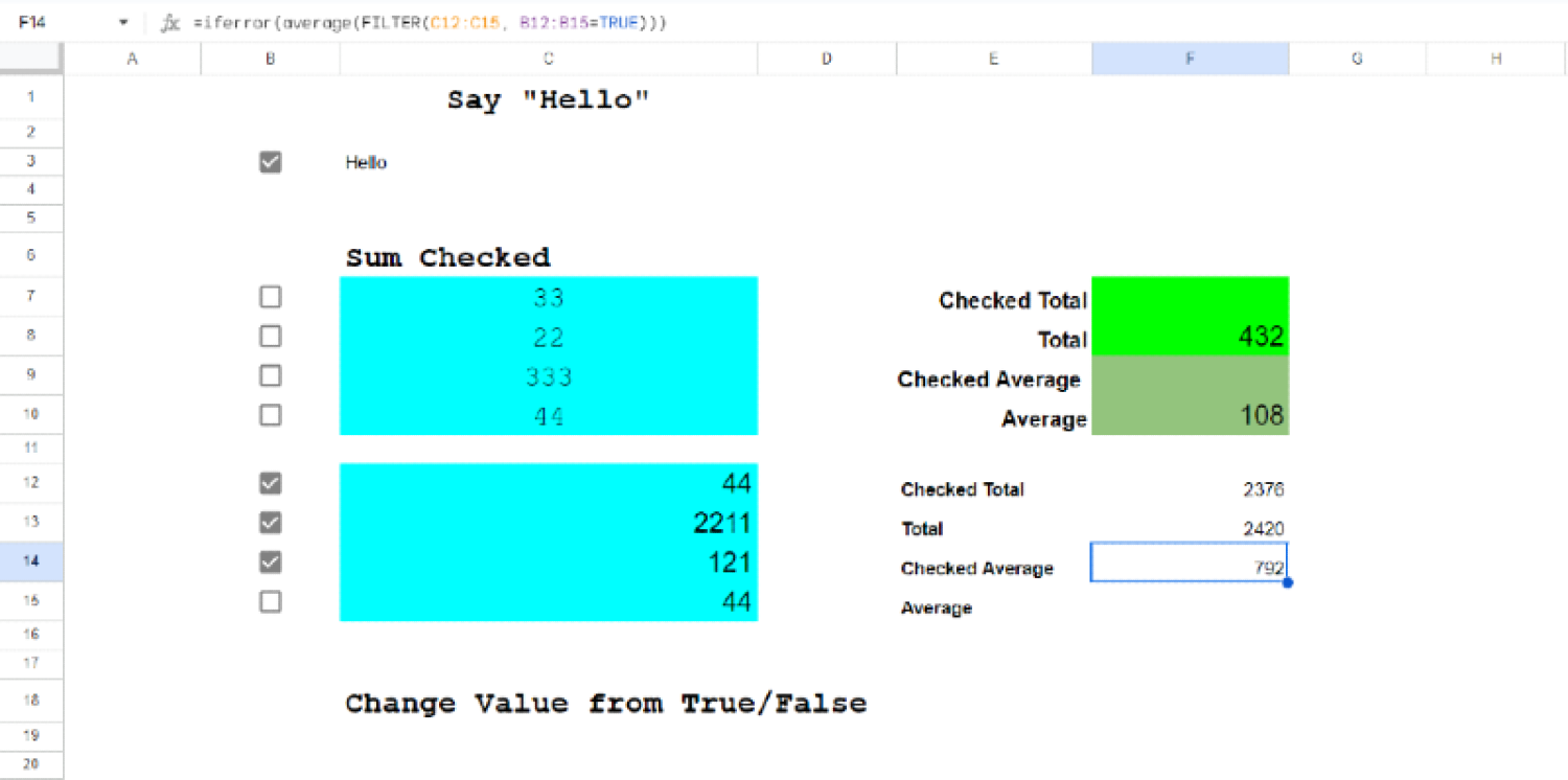
• Calculate Average. Similarly, calculate the average with the formula:

=IFERROR(AVERAGE(FILTER(C12:C15, B12:B15=TRUE)))

Doing this method, can easily help you control which data is included in your calculations, providing a dynamic and interactive way to manage your data.

4. Customizing Checkbox Values

Another thing that you can do with checkboxes in Google Sheets is change the default true/false values of checkboxes to custom numbers. This feature is perfect for creating priority lists or conducting surveys.

• Data Validation. This is how you can do Data Validation in Google Sheets:
• Go to Data tab and choose Data Validation

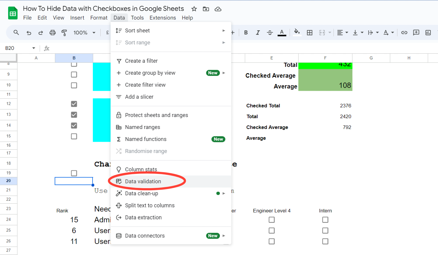
• choose Tick box under Criteria , and then check "Use custom cell values."

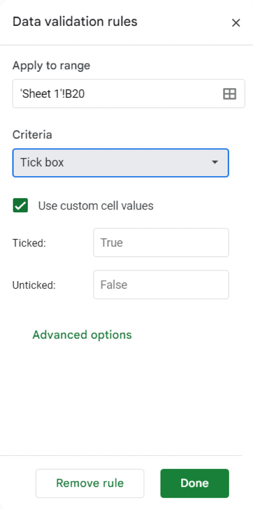
• Set Custom Values. For example, you want to set the Ticked (checked) to 1 Unticked (unchecked) to 0, or use larger numbers like 100 for checked and 0 for unchecked. Then clicked Done to save.

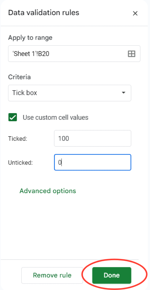
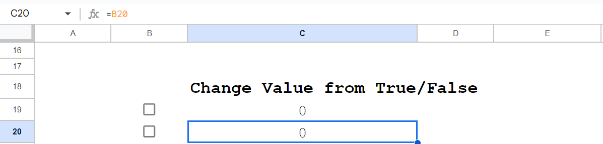
So when I put the formula:

=B20

It will show 100.

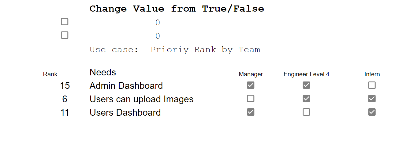
Checkboxes are incredibly useful, you can use it for gathering input and prioritizing tasks. For example, you might want to survey your team and put different points based on their level of seniority but still gather everyone's input effortlessly. You ca simply change the values and by going to Data Validation.

Checkboxes in Google Sheets are a game-changer. They add interactivity, flexibility, and functionality to your spreadsheets, making data management easier and more enjoyable. Whether you’re hiding data, summing selected values, or conducting surveys, checkboxes can make your tasks more dynamic and engaging.

Watch on YouTube