How to create a formula for every row in a column in a Google Spreadsheet?

The question asked was:

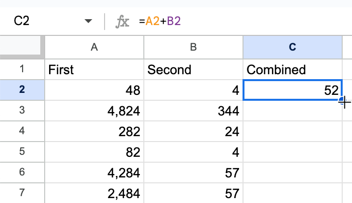
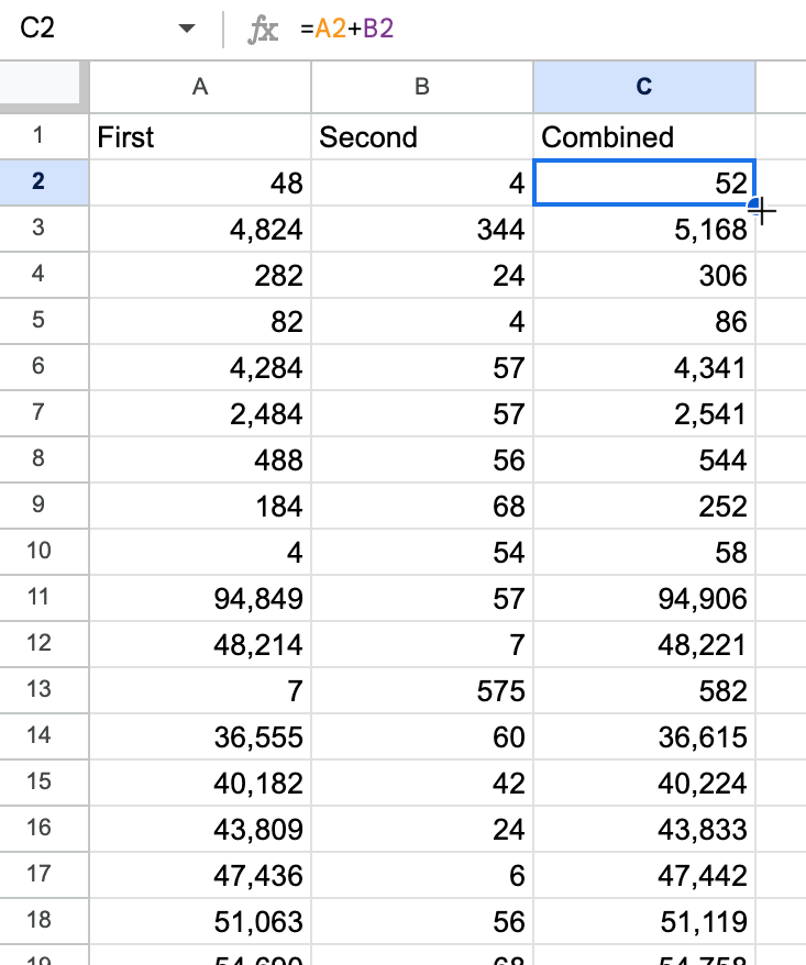
I use three columns. A, B and C. In column C I have a formula every row =A2+B2 and then for the next row I have =A3+B3 in C3.

How can I do so I don't have to type in the new formula in column C for every row?

There are a few answers to this question when using modern Google Sheets software. I've seen this question asked before, in different ways, over the years the answer is changing, and there are many ways to actually do this.

Here are 3 possible ways, with slightly different results on how you do it, but the same result in the end. (sort of).

• Auto fill
• Double Click
• ArrayFormula

Suggested Auto Fill

As you type a formula in a sheet, Google Sheets, now, is smart enough to know you might want to type that formula again in the next row, and the next. and for however many rows you have.

You're typing this "=A2+B2"

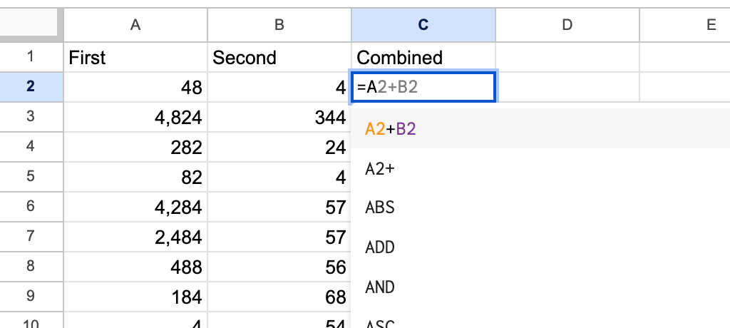
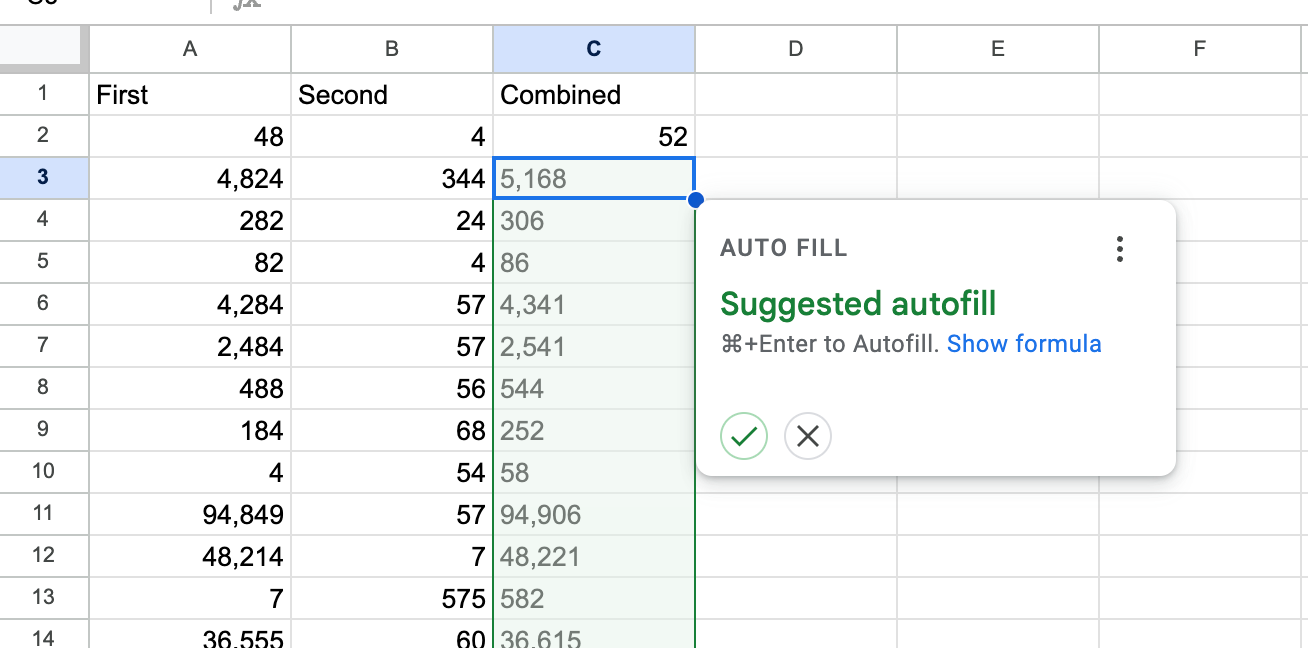
As soon as you hit enter you get an Auto Fill message from Google Sheets asking if you want to fill in all of the remaining cells that have data to the left. The reason you get this is because you have blank cells below, and the same set up as the 1st row you're typing in, to the left.

It is a "Suggested autofill" so you don't have to take the suggestion.

If you are using your keyboard and want to select the check mark which means "YES gimme gimme that sweet sweet autofill" then you can use the keyboard shortcut: COMMAND + ENTER (on a mac) and then it will execute exactly what it says here.

Google Sheets is smart, right?

But our hands... might be too fast.. we might have entered "enter". We want the data back! Have no fear, Double click is here!

Double Click

In the case that you hit enter, and not the COMMAND + ENTER to select the suggested autofill, you don't have to go back and type the formula again to get the auto fill.

Sure sure sure you can type it again in the next row and autofill might come up, but you don't have to take those steps. You don't have to wear down your keyboard anymore.

Take up your mouse, or now... probably you're trackpad.

Hover over the bottom right corner of the cell you just typed. It's got a little blue dot. Your cursor might change. That's Okay.

now Double Click.

You should then get the result of the suggested auto fill.

The rows under the formula you typed will be filled with the formula, and the relative cells will change for each one.

You have accomplished exactly what the auto-fill would have done.

And so now you think, your job is done. I have done what I needed to do.

But wait. there's a much more elegant way to do this.

there's a better way!

Arrayformula

There is a formula called ArrayFormula that turns almost any formula into a formula that can use ranges instead of just single cell references.

This means that you have to do a little editing, but it's worth it!

And I'll show you one more more "elegant" trick than almost anyone else will ever show you!

First let's tackle the "ArrayFormula" formula.

Here's what you get if you just wrap the formula you had before, with "Arrayformula".

what I mean by wrap is that you add "arrayformula" between the equals sign and your formula. Make sure to add the first open parentheses. These days you don't need to worry about the closed parenthesis. If you just need 1 more closed paranthesis Google Sheets should add it for you when you hit enter.

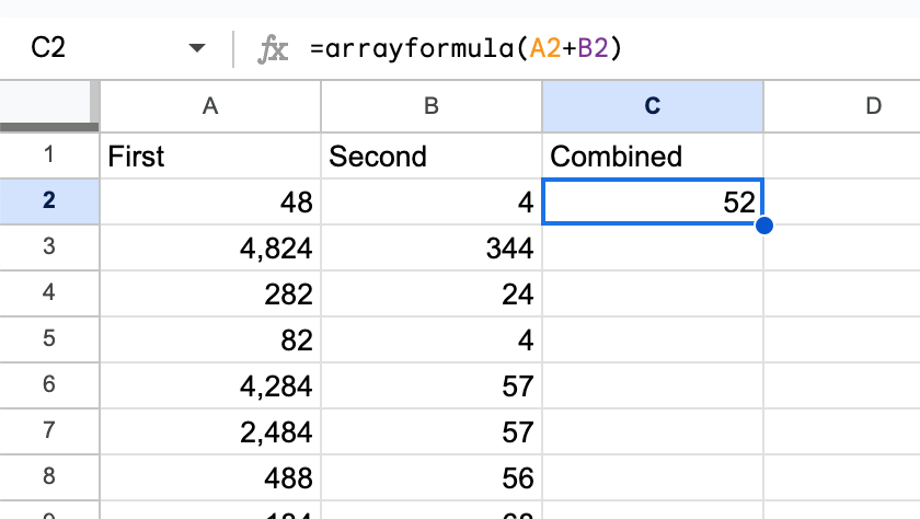
But if you do this, nothing happens.

It's because we need to manually change the A2 and B2 to ranges.

Change the Cell References to Ranges

This is probably the hardest step. But I'll walk you through it.

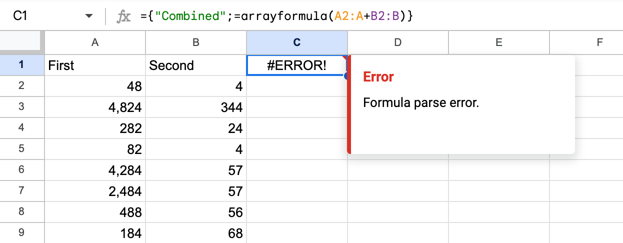
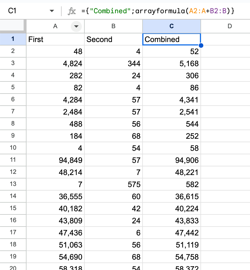
=arrayformula(A2+B2)

First change A2 to A2:A, the colon and the A means that it's a range now. Not just a single reference to a single cell. The colon always means from this one to this one. We're going from A2 to A.. but wait what's A? that's shorthand for the whole column.

Yes you absolutely can do a smaller range: A2:A10 for example.

But let's just do the whole column.

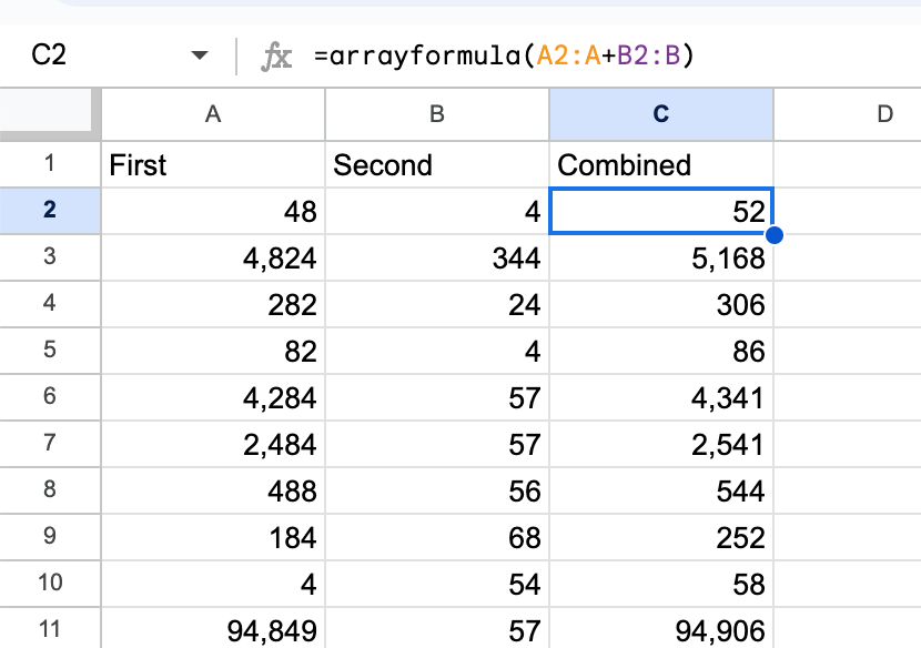
=arrayformula(A2:A+B2)

And now do the same change to B2.

We'll edit B2 to be B2:B, or B2 colon B.

=arrayformula(A2:A+B2:B)

And that's what we did here in C2.

so in C2 is the array formula and it fills out the whole column.

but if you go down the bottom, and see where the information to the left is blank. The array formula keeps going.

You can easily fix this by wrapping the content of the ARRAYFORMULA() with a formula combination of IF() and ISBLANK().

the syntax will be essentially :

IF(ISBLANK(A2:A),,<what you want to display>)

I'll show you here.

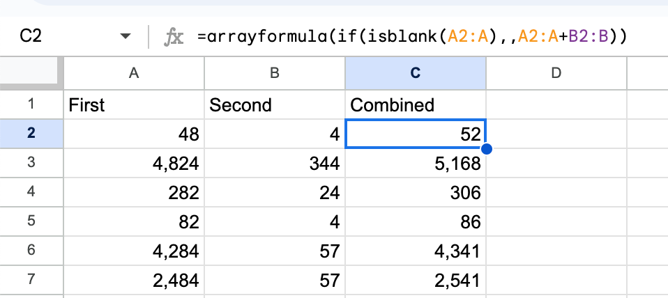
Make sure you change make the cell reference inside of ISBLANK() also a range, with A2:A.

But you don't have to do that part all the time. You can leave the formula as is, and you'll have a column of zeros in this case.

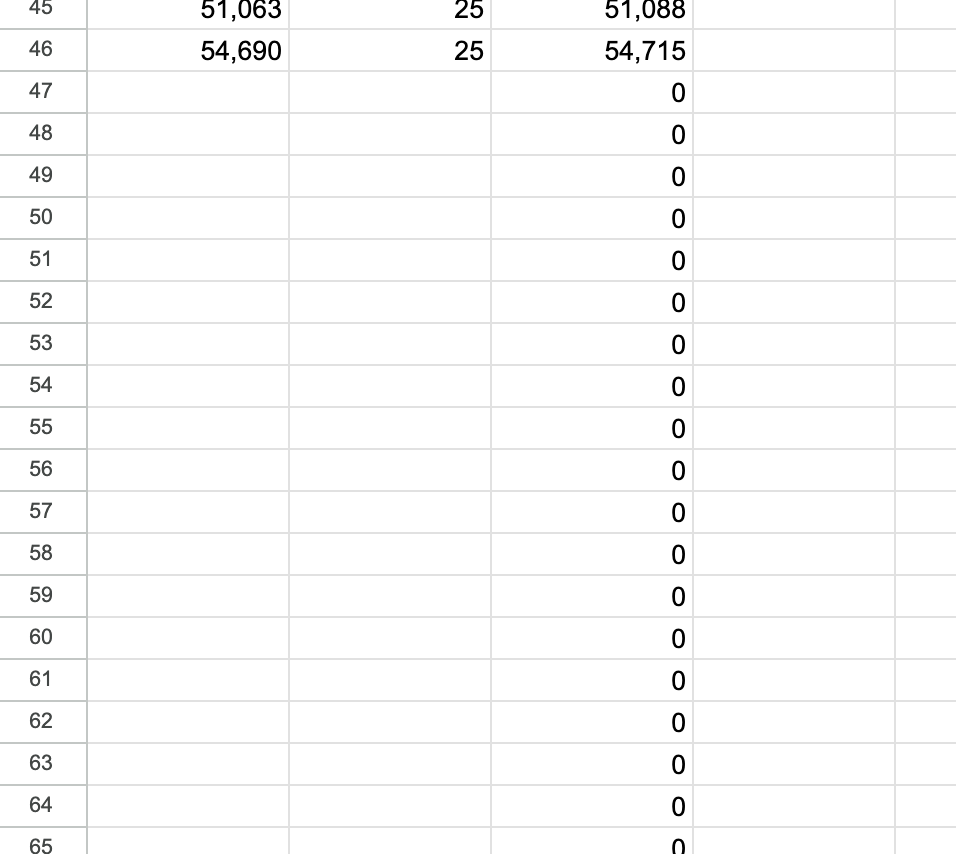
Which aesthetically speaking is not the worst thing. Because you can see that a formula will have a result there once you add the data in the A and B columns. If you had some other formula that resulted in an error then this hiding the results unless the data is there would be very useful.

Let me show you one more trick.

One More Trick!

You can add the arrayformula to the header line if you would like to have the data rows without the array formula in there.

Yes you can. You can really put the arrayformula and the header text in the same cell. I'll show you!

The way you have to do it is to wrap two elements in curly brackets. And then you have to use a semi-colon as a delimter. Or rather have the semi-colon separateing the elements in your curly brackets.

Those two elements are the header text with quotes, and the ARRAYFORMULA.

It will be like this:

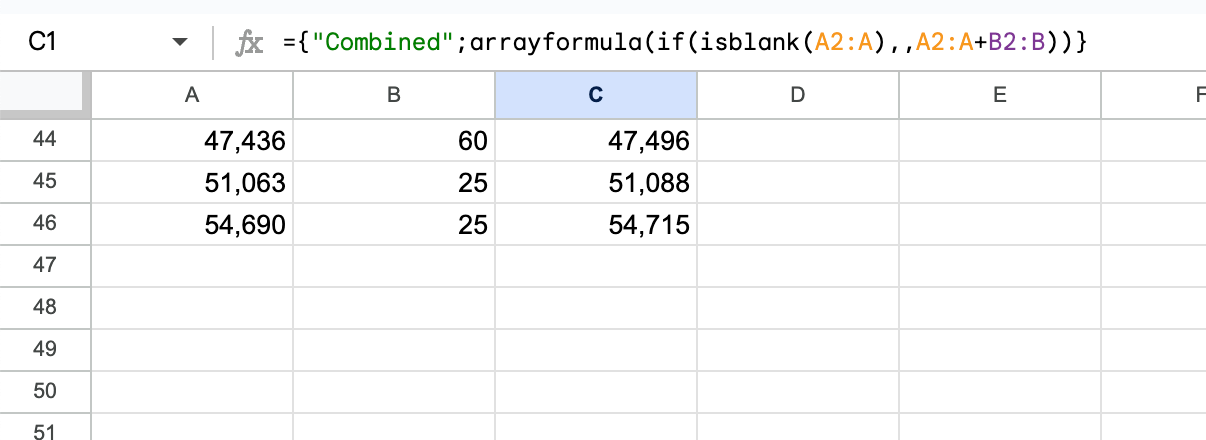
={"Combined";arrayformula(A2:A+B2:B))}

If you try to copy paste the whole arrayformula formula you made into the curly brackets, you might accidentally include the equals sign. If you do that you'll get a formula parse error.

This is the end result. the text Combined is vertically listed before the ARRAYFORMULA.

Google sheets then renders the ARRAYFORMULA which will extend down the entire column, in this example.

If you had set the range to something like A2:A10 and B2:B10 then the result would go until row 10.

And it is absolutely okay to combine these two techniques. You can use the curly brackets with the IF() and ISBLANK() combination.

This way you get the best of both worlds, your cells have the result and...

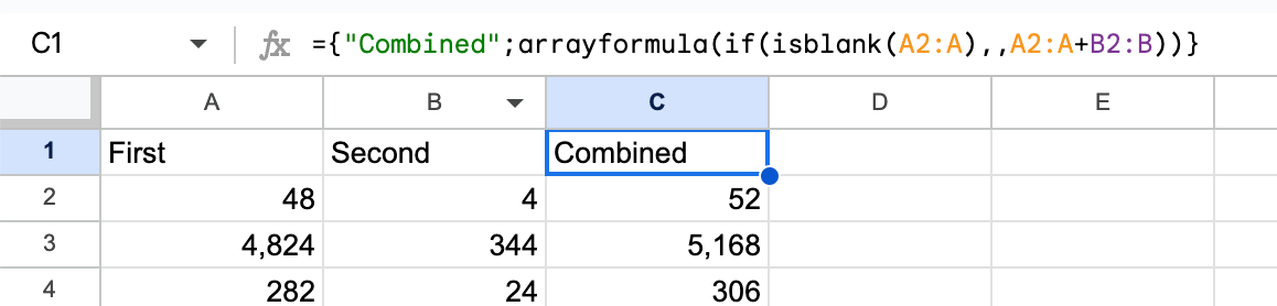
When you have no data for the formula you don't get a list of zeros.

Wrap It Up

When you're trying to create a formula for every row in a column in Google sheets you can use Google's auto fill. If you miss that chance, you can also double click on the cell, as long as you have the data already in the cells that you're referencing.

And if you would like an approach with formulas, use the ARRAYFORMULA() formula.

In this post I showed you to ways to make the result better. You can add the IF()/ISBLANK() combination to hide the extra cells of data at the end of your range.

And you can add the ARRAYFORMULA() to your header so that you don't have a formula in your data.

More Formula Combinations

If you liked seeing the IF/ISBLANK formula combination, Better Sheets features video tutorials of all kinds of fun, funky Formula Combinations.

Automate Your Sheets

You can automate sheets with formulas alone. At least they feel like automation. I feature more of these kinds of formulas that feel like automations in a free YouTube video. But if you really want to learn how to automate your sheets, take Spreadsheet Automation 101. Featured on Udemy.

And also is free for all lifetime members of Better Sheets as well as monthly members.