How can I count true and false?
Master the art of counting 'true' and 'false' in Google Sheets with this detailed guide. Uncover pitfalls to avoid & learn powerful functions.
In this tutorial, we’ll answer the question, “How can I count true and false or true or false?”
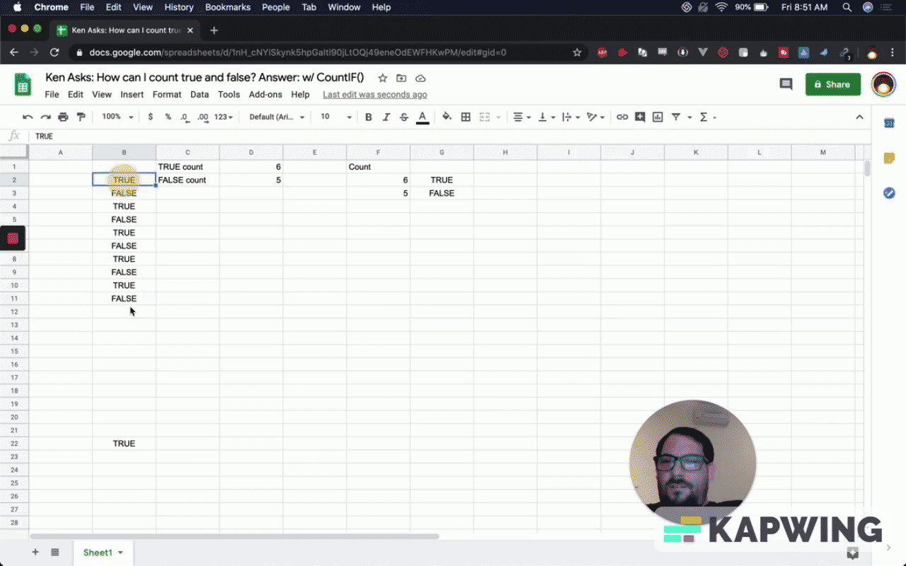
The answer is if you have a column of true or false, you can use the =COUNTIF() formula.
That's just =COUNTIF() and then you enter your range and then comma, True or False, whichever one you want and you'll get a count.
If you notice, I have all these true down here (in the spreadsheet). I've used lower with quotation marks in true and it's not counting them. It’s like knows that the term true should be all caps true.
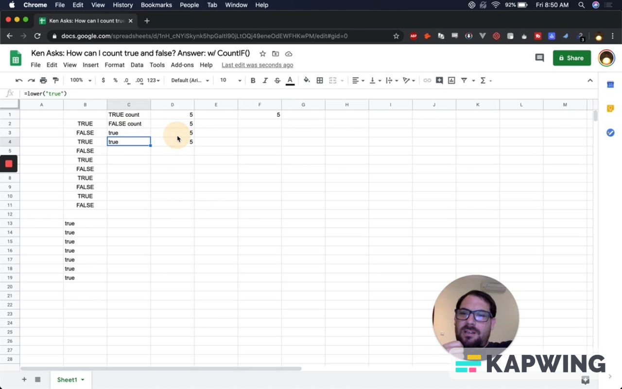
When you type in true, it actually redos it as all caps true. It doesn't count all lowercase true.
Even if I put as the argument that this lowercase is true, it's not counting it in the formula. It thinks that all lowercase true is all uppercase true. It’s a boolean statement, which is true or false or one or zero.
It’s a very interesting pitfall you might run into. If you have the text true in all lowercase, it will be counted. If you have true or false, it will be counted even if you use all lowercase true and the =COUNTIF().
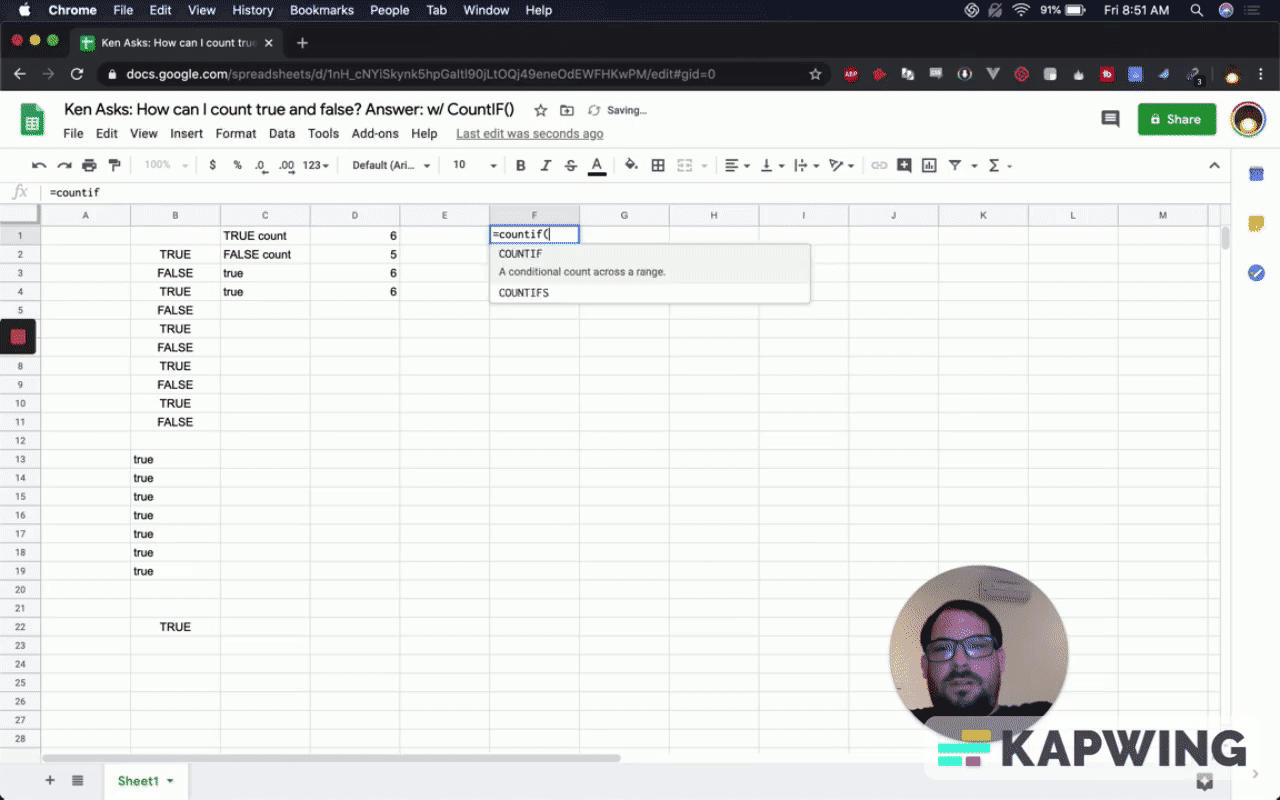
Instead of writing the word true or false, here you can say =COUNTIF(), put in the range, and put in G1. So now it's counting this and you can just put true there. You can also put false and now you have a counting.
You can use a checkbox and check boxes are only true or false. Highlight the true or false (B2 – B11), click on “Insert” found in the menu, then insert checkbox.
It automatically knows that True is a checked checkbox and False is an unchecked checkbox.
Let's say I'm going to insert check boxes here (D6-D14) and then insert some data (E6-E14). We want to check this, right?
Delete the data under column F (F1-F3) and G2-G3.
Create a new Count header in F6, so that it’s within the area of our new checkboxes and list of data.
Type in true and false in G6 and G7.
Enter the formula =COUNTIF() in F6. Your range should be D5 to D14.
It should have all trues, which is G6.
=countif(D5:D14,G6)Now we have zero.
And how many False do we have? Nine.
(You can watch the short clip below for the steps mentioned above.)
You could also use a checkbox as a true false statement and you can use them in inter-operably meaning you can replace them with each other.
So if you already have a column of true and false, you can replace it with checkboxes to make it one click true or false.
This is interesting. If you have checkboxes already and you want to change them, you can use the equal sign. Now you have a true/false from a checkbox programmatically.
Check for true. Uncheck for false. Count true, count false with the IF formula.
You can use these true false statements inter-operably with checkboxes as well, and then count checkboxes in the same way.
And that is how you can true and false. You can also do something extra with checkboxes.
Watch the video for this tutorial:

Learn from other questions about Google Sheets:
Get more from Better Sheets
I hope you enjoyed this tutorial! If you want to do more with your Google Sheets, I have other tutorials, like how to create a timer with Apps Script and learning to code with Google Sheets. Beginner? Intermediate? There’s a lot of tutorials for everybody! Check them out at Bettersheets.co.
Join other members. Pay once and own it forever. You get instant access to everything: All the tutorials and templates. All the tools you’ll need. When you’re a member, you get lifetime access to 200+ videos, mini—courses, and Twitter templates. For starters. Find out more here.
Don’t make any sheets. Make Better Sheets.