Filter a Database in Google Sheets based on Dates, Checkboxes, and Dropdown selections!

In today’s tutorial, we’ll be answering the question from Mohamed. The question is “How do I filter a database in Google Sheets based on dates, checkboxes, and dropdown selections?”

The actual problem is he has a list of cars. He wants t filter out everything that is outside of the start date and end date. I'm not sure if these are particularly the date of sale or date of creation. There is a little bit of interesting thing you can do with dates.

What you'll get when you finish this tutorial

With this tutorial, you’ll learn how to filter everything that is outside of the start and end dates. It’s basically learning how to filter between two dates.

You’ll also learn how to filter different situations using checkboxes.

Are you ready to learn something new today? Let’s get started!

Two particular problems

There are two particular problems here. He's asking for a car type Nissan only or Nissan and Toyota. In order to solve this challenge, there are a few ways to deal with this. It's just a little complicated question because the answers are vastly different. I'm going to get through this as best I can with the information I have. It’s absolutely understandable if this is not the correct answer.

The very first thing I'm going to do is I'm going to create a list of cars with these kinds of data. I'm now going to show you how to set this up.

Setting up the database function

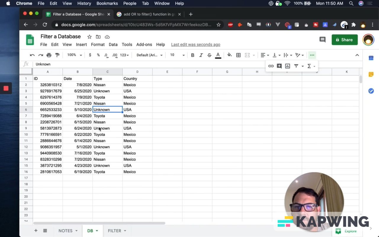
The first thing we have is a database.

He's asking for a database function where you have the table of raw data. You see everything, including the bar above that you can filter.

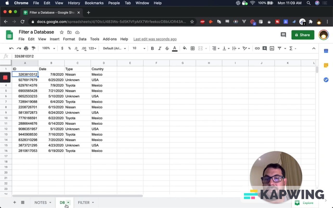
First, have to have a database on a separate tab so that you can filter. I've created that tab. I've also created IDs so we know what we're getting.

We're getting some other information other than just the type and the country. I've added Mexico here and some other countries. These are totally random.

I don't know if this is a data sale or date of purchase or anything else, but we had some random dates here.

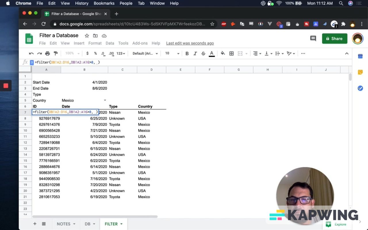
Now let’s go to the “Filter” tab; Type the following formula:

=filter(DB!A2:D16,DB!A2:A16>0)

We’re going to get everything for this formula to work. We need to filter something. We want everything under the ID column.

For the part with 0, that's going to need to be the same thing. Basically, it needs to look at the exact same range, so your database and your filter need to be the same thing there or you'll get an error.

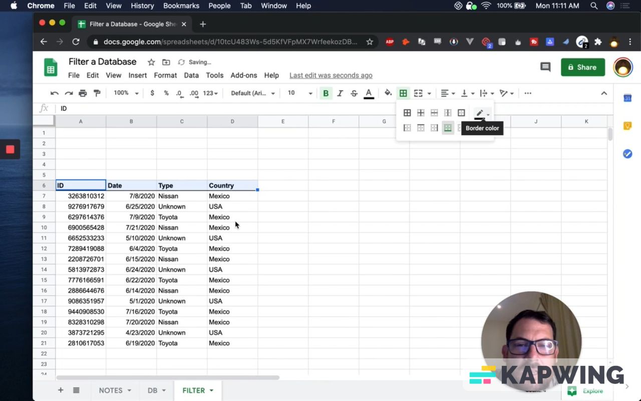
We have everything we need now. Don’t forget to put the headers, like ID, Date, Type, and Country.

You can put a line under the headers and hide the gridlines.

Now we want to filter.

Input Start Date and End Date first. We're going to be searching between those two dates, so add a couple of dates.

The next thing we want is to add the type and then be able to select the country.

If we want to make a dropdown menu, you'll see this in “List from a range.”

We are going to go back to our database and we're going to select country and save it.

We can definitely fix this dropdown menu in the “Country” field.

This is the hardest part of this entire tutorial: Selecting multiple types of cars.

Let’s go through the filter of Start Date and End Date first. Then we’ll come back to “Type” field

In order to filter this by these dates, here's what we need to do: We need to add two filters.

We already have only the ones with an ID.

Then we add a column.

We add the second part, which is the one in blue text in the screenshot below:

What that means is we'll include everything with a Start Date. You can do not the minus one, and then you'll get everything in the between – which does not include the Start Date.

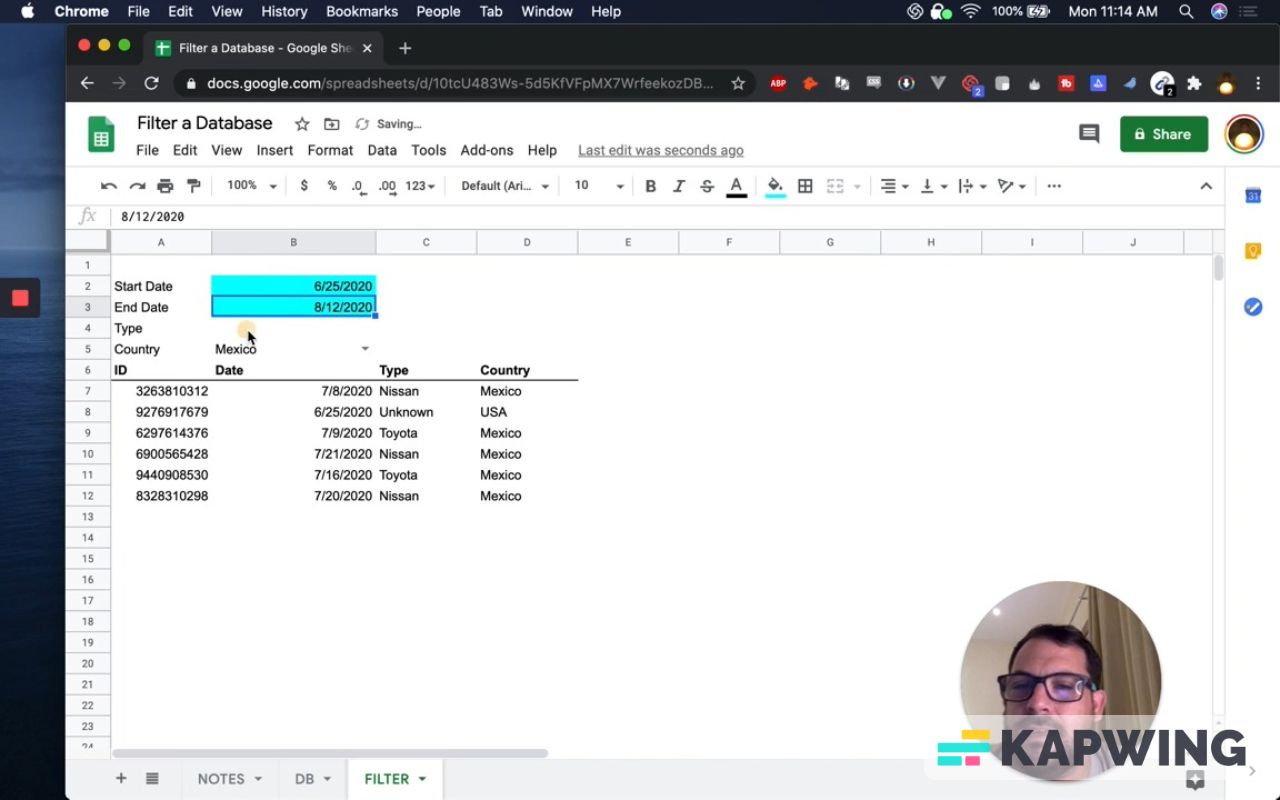
Let’s double check. Let’s bring the Start Date to June 10th and see those things that disappeared. Now everything is between June and August 6th.

What we’re doing here is filtering the database tab, where we can add anything, for the Start Date and End Date.

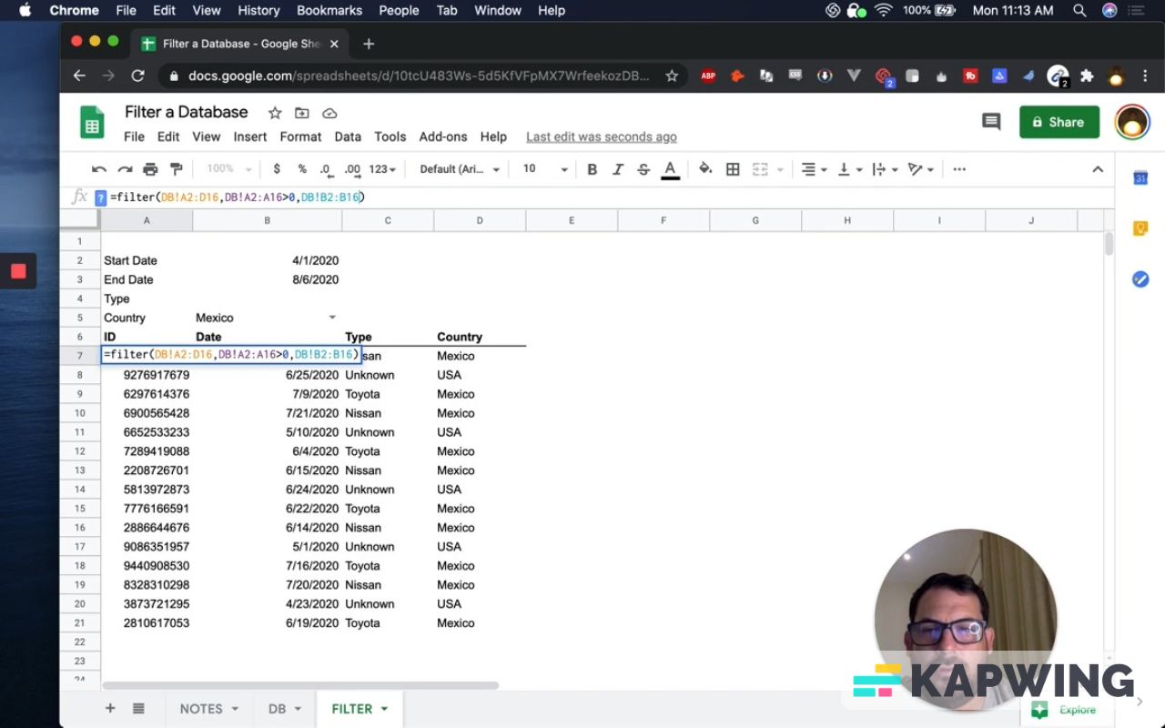
Now we need the country.

Let’s add the formula for the country. It’s the last one in yellow text with “B5” in green.

<=B3,DB!D2:D16=B5)

Now everything other than Mexico shows up. And if we use USA, now we have USA.

Why do you need to create your own filter?

The built-in filter has a lot of options available for you: You can filter by color or do sorting plus filtering. But what's interesting is that sometimes, in some cases, you do want to have a filter that you design your own way but you have limitations and opinions.

Why I don't use this built-in filter almost ever is because by using it, anyone else using this document now sees this filter and is only able to see what's in the filter. They must turn the filter off and then they can see the data. It turns the filter off for everyone viewing this sheet.

By building your own filter, what you're able to do is be opinionated and set things how you want to set them. What you can also do is create this filter on a completely separate worksheet and give people different views into the same data.

You can even set the filter and then duplicate it. Now you can set a different filter where you can give different views to the same data to different people. If you only want to see everything from the last seven days, you can do that with this kind of filter, too.

But then this data is only available to see, be seen in that. By adding your own filters, you can see it in different ways.

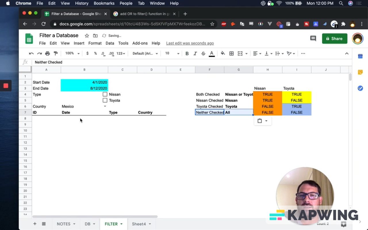
Here are four situations that we have:

1. Neither is checked = We want to see all.
2. Nissan checked = We only want to see Nissan.
3. Toyota checked = We only want to see Toyota.
4. Both checked = We want to see Nissan or Toyota and nothing else.

Watch the video below to see the situations in action.

We have unknowns in our DB tab, right?

What happens is an IF function has three arguments. It has something that is going to resolve true/false.

What’s interesting is if you insert a checkbox. The checkbox is literally a visual representation of the values true/false.

If you check on it, it is true. If you uncheck it, it is false.

We’re going two have two arguments: True and False.

The values remain the same: If it is True, it is checked. If it is False, it is unchecked.

Then in our IF function, we use this formula:

=if(C3,D6,E6)

C3 = checkbox
D6 = if it’s True (checked)
E6 = if it’s False (unchecked)

String together the three arguments

There are three arguments, but we can string these together to get a variety of things.

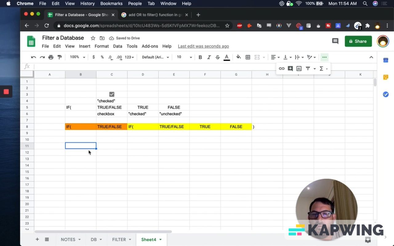
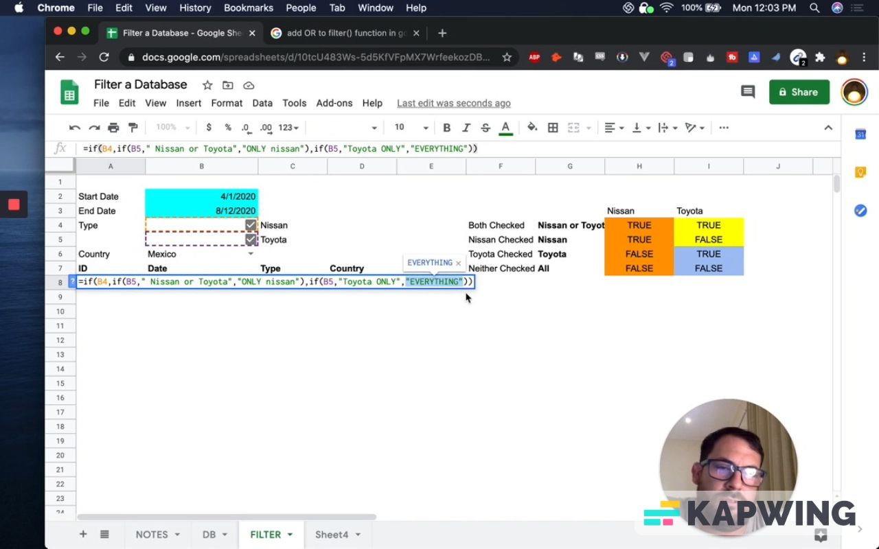
In B8, we start with IF( and then use our checkbox with TRUE/FALSE in C8.

If it’s True, do another IF in D8.

And now, inside of that TRUE, do TRUE/FALSE in E8.

Do TRUE in F8 and FALSE in G8.

Then end the formula with a closing parenthesis, which is “)” in H8.

To make things easier, let’s color the first TRUE/FALSE orange and then color the other TRUE/FALSE yellow.

Then we add the following:
• Comma in I8
• IF( in J8
• TRUE/FALSE in K8
• True in L8
• False in M8
• Closing parenthesis in N8

Let’s color this blue.

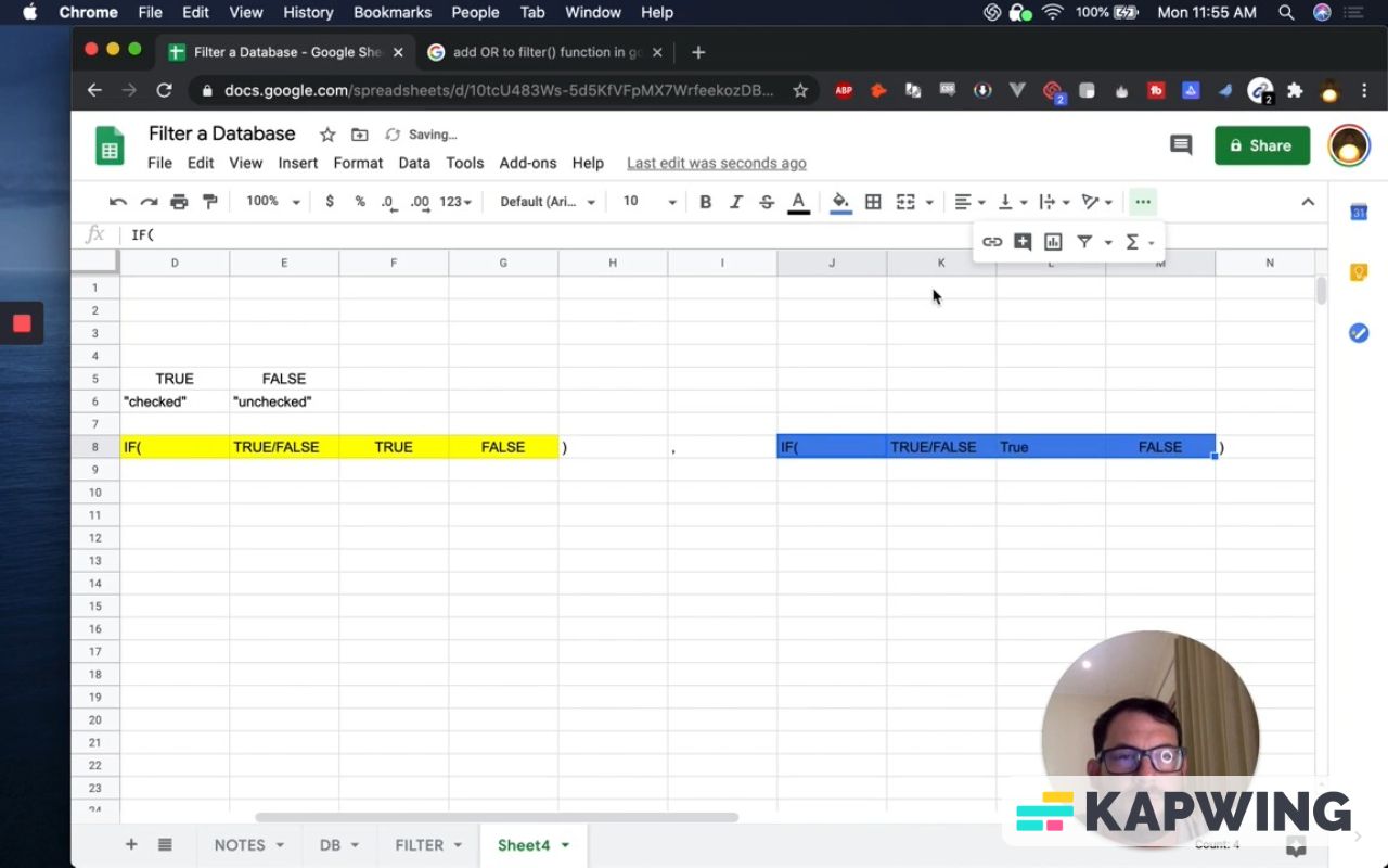
Let’s start using these TRUE/FALSE with their corresponding colors so we can have a more visual idea of how to use it.

Here are the situations:
• All orange = True, True, False, False,
• Yellow = True, False
• Blue = True, False

Here’s a video clip for to make it more visual :

Let’s go back to the FILTER tab. I think that gets us our all of our options here.

Again, I do believe this is not the only solution. There might be some very quicker solutions, faster solutions, but this is a solution I've gotten here.

First one we want to know is Nissan, check. We want True, False – Refer to the screenshot above for a visual reference.

If B4 is True and B5 is False – meaning we have Nissan Check – we don't have Toyota Check, then this is only going to be only Nissan.

Now we have the other side. If B4 is false and if Nissan is checked, then we need to know, “Is Toyota checked?”

Now you can see the different situations in action:
• Everything. = both are unchecked
• Nissan is checked = only Nissan
• Nissan and Toyota are checked = Nissan or Toyota
• Toyota checked = only Toyota

Now we just need to figure out what we put in the filters.

The easiest filter is All, which is “Everything”, so let’s start with that.

We don’t care about the C column at this point. It’s just going to be “Everything.”

Let's just uncheck it and double check that there's everything. It’s everything based on the other options, like Country.

Let’s do Toyota now.

Where it says “Toyota only”, we're going to copy our filter again. In this case, we will do C5 and now if Toyota is checked, we only have Toyota.

Let’s do Nissan next.

We'll copy and paste “Only Nissan.”

Now our C column is C4. That is correct.

So now just that check. We have only Nissan.

The last thing we need to figure out is Nissan or Toyota.

How do we have a filter where we have both of those?

A simple answer is that we put in curly brackets in both of the filters.

Start by deleting “ Nissan or Toyota” and then put in two curly brackets, like this:

=if(B4,if(B5,{},

And within those curly brackets, we’re going to put in a filter, a semi-colon, and then another filter.

Then we’re just going to change the C4 to C5.

So now we have two filters in there, and the curly brackets put those together.

I'm not sure if you absolutely caught it or if I showed you, but in curly brackets, if you put two things together and one of them has an error, the entire thing has an error.

But in this case, we only get to the point of having them in curly brackets when we know it's completely true.

So now we have:
• different situations of True, False
• our filter functions (Start Date and End Date)
• our Type (Nissan and/or Toyota)
• our Country

This is really cool! Hopefully, you now understand or at least see an example of a very complicated filter where we have different types of situations where we have checkboxes as well.

Instead of just a filter based on exactly the date, we have greater than or equal to the start date and less than or equal to the end date.

Then we have our country filter that is based on a dropdown.
If this is confusing at all, feel free to comment down below what your frustration and challenge are and I'll try to make a follow-up video/tutorial based on clarifying that situation.

Watch the video for this tutorial:

Better Sheets Google Sheets Tutorials, Templates, Tools, Tips and

Learn more about Google Sheets:

Get more Google Sheets Tutorials at BetterSheets.co

We love Google Sheets here. If you love Google Sheets as well, you might want to consider becoming a member of Better Sheets. For only $19/month you can access over 200 Better Sheets tutorials. Learn Apps Script in under 40 minutes. Design better dashboards. Make your sheets faster and yourself more confident in sheets.