Create a Many to Many Database inside Google Sheets

In this tutorial, I’ll show you how to create a many to many database inside Google Sheets. If you ever ran into the problem of wanting to put multiple categories into just one cell, you’ll want to keep reading below because that’s exactly what I’ll teach you.

For this tutorial, our example has a list of names and lead categories. But what we really want to do is put all of that information into one cell and show it right next to this person.

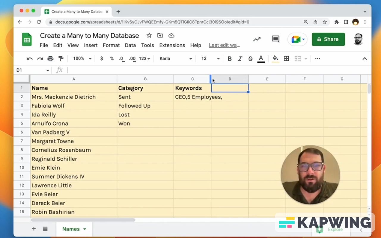
In the case of the Lead (column B) there's only one. But in the case of Keywords, there might be many. There are different types of companies that you're reaching out to or different types of people and, and people have more than one category or keyword that they're a part of. For example: People can be both a mother and a CEO or a father and a CMO.

One of the problems you're going to be facing is if you're trying to fit in everything into one cell and you're doing it manually. You'll know the problem you're facing when you're adding comma separated values into one cell and you're like, “There's gotta be a better way than typing these in or select.”

There's gotta be a better way.

There is. The thing is you have to do a couple of things to your sheet.

First off, we're going to create a duplicate of this sheet, “Names.” And instead of names, we're going to call this new duplicate “Keywords.”

So what we're going to do is we're going to take out everything, every column except for one. These are just going to be keywords. These are all the keywords we could possibly have, and we can always add to them later.

We have different things or statuses that can be combined. Here's where the magic happens!

We're going to create one more sheet. We're going to duplicate it, and we're just going to call this “DB.”

We need two columns and we're going to need no data. You can delete everything in the DB sheet.

What we need to do on the left side is to create a dropdown chip.

We're going to create a dropdown from a range, and that range is going to be “Names!A:A” Click on the “Done” button.

We're going to also copy this and paste it all the way down, so we have dropdowns everywhere.

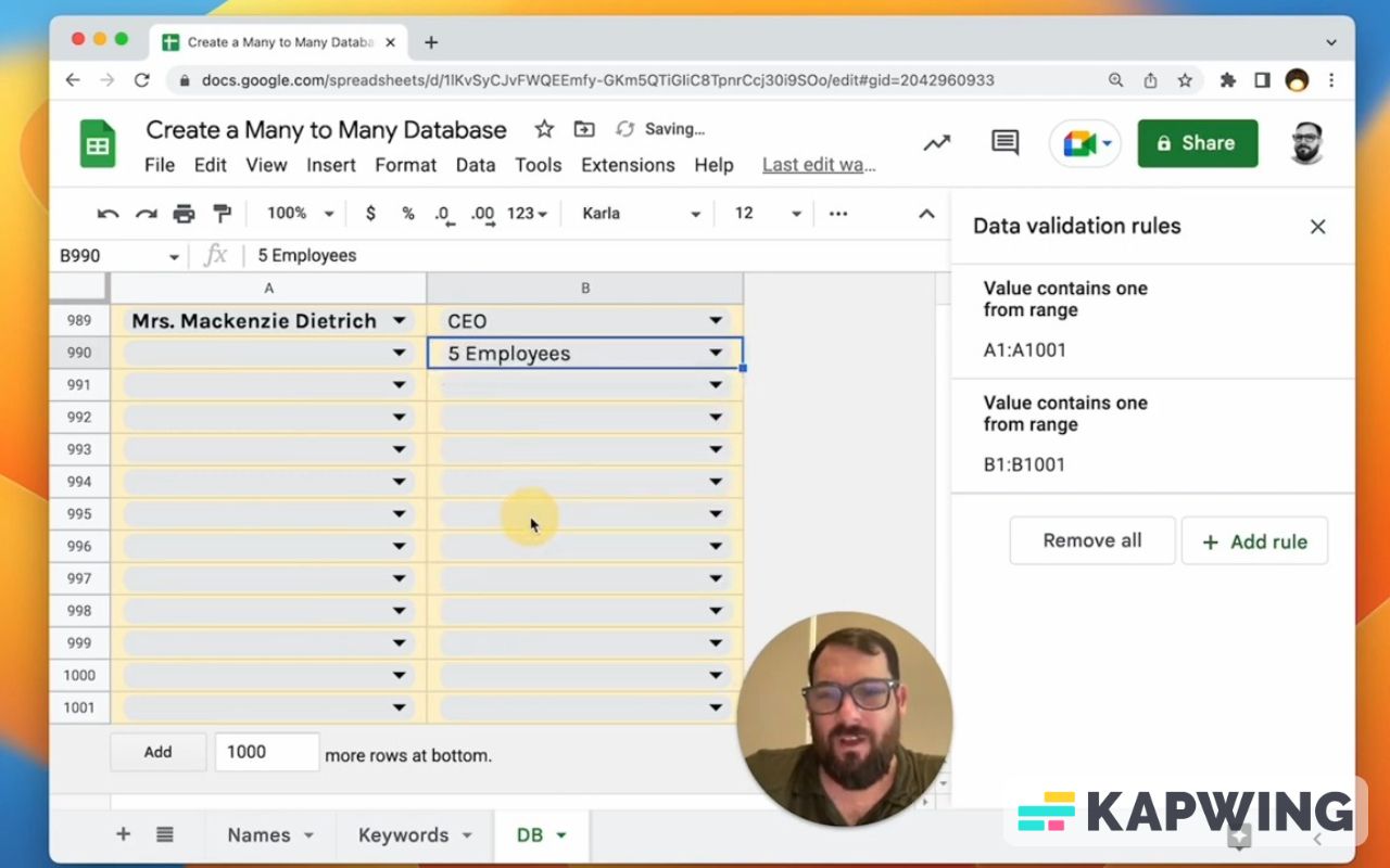
In the second column, the B column, we're going to do almost the same thing. We're going to insert a dropdown, but in this case, we’ll choose the criteria called “Dropdown (from a range).”

We're going to enter “Keywords!A:A” in the field below that.

And again, we're going to copy that one, drop down all the way down to the bottom. There we go!

So now we have two sets of dropdowns from ranges. One on the left side, which is our names. We can select someone like Mrs. McKenzie. Then we have keywords like CEO and five employees for column B.

What we need to do to combine these two groups is for everyone we want to add whatever relation we want to add, we just put them next to each other.

Examples: Mrs. Mackenzie Dietrich is both the CEO of a company with five employees. Fabiola Wolf is both the CEO of a company with 10 employees.

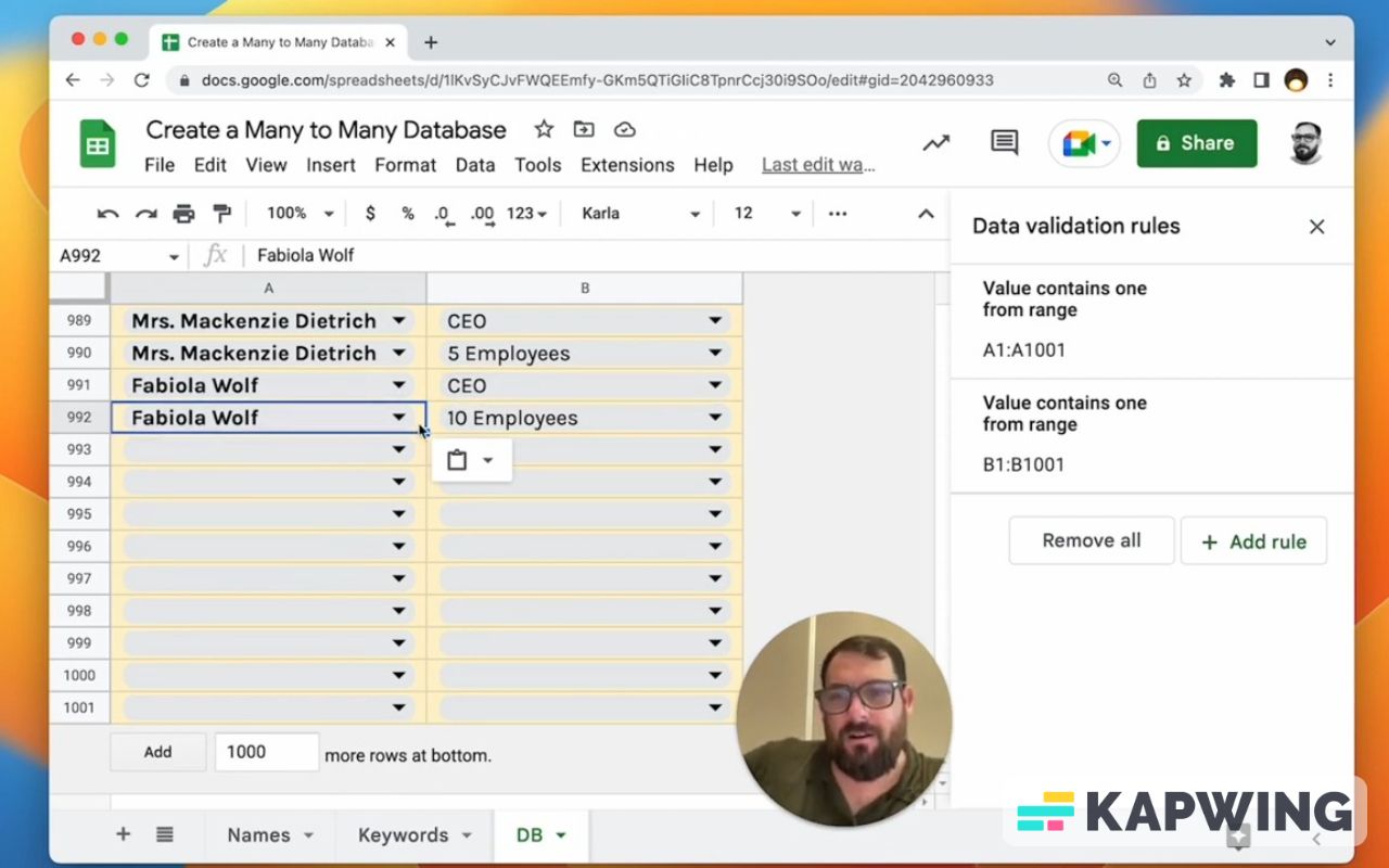
Order here doesn't necessarily matter. What matters is that you have the relation across a row.

Now we have to actually perform a little bit of magic here on our names.

The goal of this is that we want all of the keywords in one cell to be displayed here. So how do we do that?

You might do FILTER. What we need to do is this:

=FILTER(DB!B:B,DB!A:A=A2)

Let's just do this and show what happens. We get two things and it goes across multiple cells. We don't want that. We want them all in one cell.

What you might have already been doing is something like this:

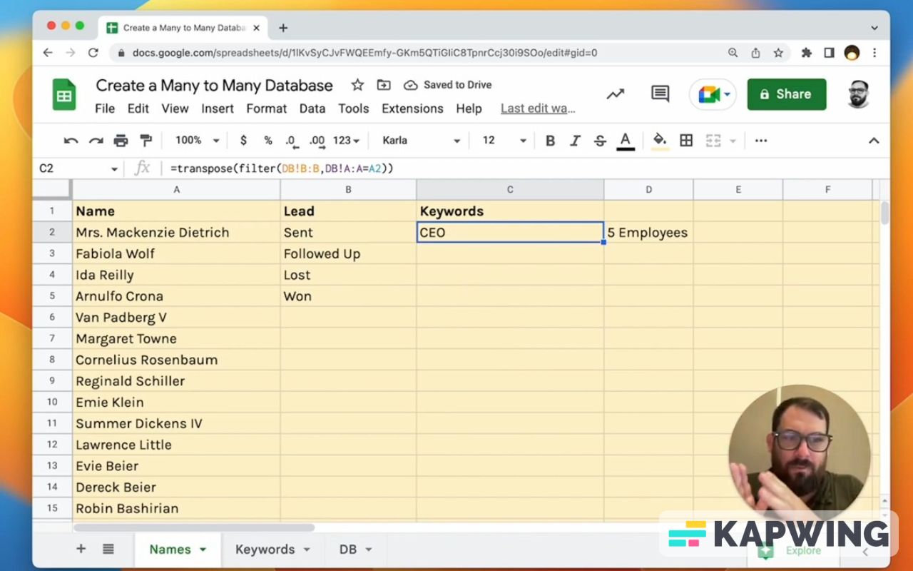
=transpose(filter(DB!B:B,DB!A:A=A2))

What this does is it just takes the vertical list and makes it horizontal.

Again, it’s problematic because our keywords are across many cells.

And maybe there's other data we have here. We want everything in one cell, so we need to do a “join.” We can join any delimiter.

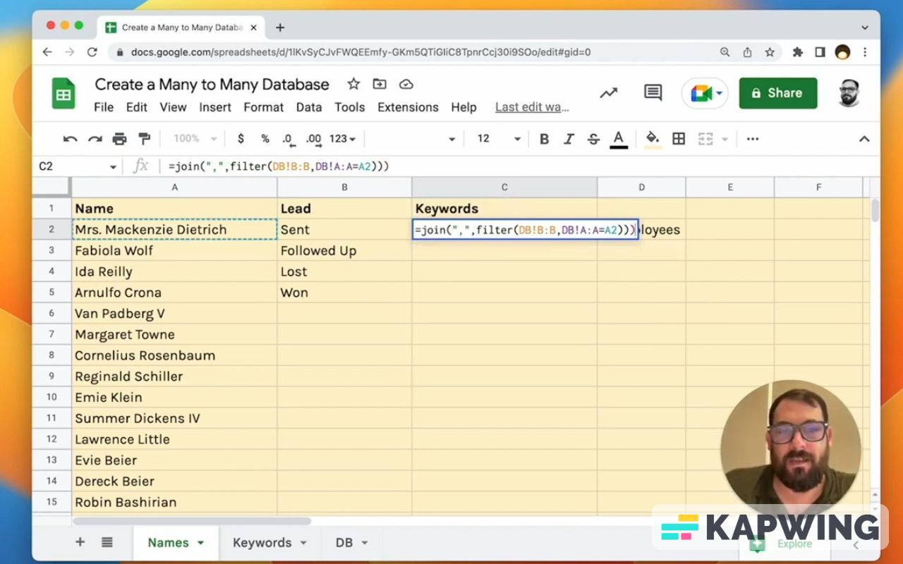
All of our values are going to be the filter that we searched for.

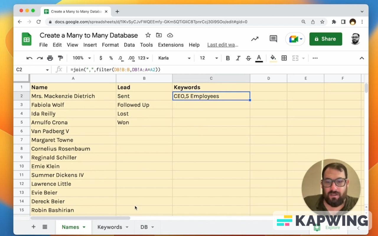
And now, in one cell, all of our keywords – no matter how many we have – are joined together.

We can add more data in our DB sheet and it gets automatically added to the Keywords column. The same filter can be copied down.

One thing you're going to get is probably #N/A and we can fix that by wrapping this with “ifNA.”

=ifNA(join(“,”filter(DB!B:B,DB!A:A=A2)),)

And there we go. We got nothing. If we have nothing, no filter. The #N/A is saying no match is found.

You can also have some text there as like no keywords found, or add some keywords, no key words. So you can have some text there, but you also might just want nothing or you can have a command that says, “Add key words.”

Now this entire database of the DB is completely manual. We can add information here as we want.

This keyword column is automatically added and it's all in one cell. It's all in one column. No matter how many keywords we have, they'll all be added and joined by a comma.

Thanks for reading this tutorial and I hope this helps you create a many to many database in Google Sheets.

Watch the video for this tutorial:

Improve your Google Sheets with these free tutorials:

Get more from Better Sheets

I hope you enjoyed this tutorial! If you want to do more with your Google Sheets, I have other tutorials, like how to create a timer with Apps Script and learning to code with Google Sheets. Beginner? Intermediate? There’s a lot of tutorials for everybody! Check them out at Bettersheets.co.

Join other members. Pay once and own it forever. You get instant access to everything: All the tutorials and templates. All the tools you’ll need. When you’re a member, you get lifetime access to 200+ videos, mini—courses, and Twitter templates. For starters. Find out more here.

Don’t make any sheets. Make Better Sheets.