Automate Google Sheets without Apps Script, without Zapier

Recently, I've been doing a lot in spreadsheet automation using Apps Script. But I wanted to go back to some formulas that I think feel like magic.

It feels like automation

They make me feel like a wizard... without having to code.

"Automation" means that if you as a user or another person using your sheet take some action or enter some data, something happens based on that action. It’s an action and an effect.

You don't need to know how to code

We can do a lot of this in Apps Script, but if you are uncomfortable with code, with diving into App script using OnEdit and OnOpen and these sort of built-in functions and you're not really convinced you want to learn to code, I want to give you some interesting formulas and formula pairings that help you make essentially automation inside your sheets. They will at least seem like automation or seem like magic sometimes.

You also don't need to read. Watch this tutorial on YouTube.

Formula pairings for that magical feeling

IF() + a Checkbox or ISBLANK()

We’re going to create literally something out of nothing.

FLATTEN()

Flatten takes a bunch of like mangled data and turns it into a single array. oooh.. let's see it in action.. later.

IFERROR() and FILTER()

These are really cool because you can set up filters before you know someone's going to fill it out and then, as if like magic, their information is filtered.

TRANSPOSE() and UNIQUE()

This combination can create headers.

IF() + Checkbox

The simplest way I can show you this is if we create like a to-do list. There’s a task list inside of sheets and we have a checkbox. Coolest thing about checkbox is that they are a visual representation of the values of true and false.

We use =IF logical expression in our if formula. Remember: Checkboxes are True or False. If the value is true, meaning it's checked off, it'll show something. If it's false, it'll show something else.

One thing you can do in this particular case is this: If it's true, write a word, and if it's false, we can say something like “Task 1.”

What that allows us to do is when we hit this checkbox, this is done.

We can also conjure it from nothing. We can write this all the way down. We can also put all of these tasks on a separate tab and then reference their cell here instead of the word task one. We can reference a cell like B2.

Now we can see that this is done right. It changes our text just based on that action of checking off.

We can also show things. So let's say we don't want to see task two through 10. Basically, we don't want to see the next task until we're done with one.

For Task 1, we’ll leave the formula as is. For Task 2, we’ll do this:

Our logical expression is going to be the row above it, A2. We're going to say if the value is true, show Task 2. If it's false, meaning there is no check mark.

We are going to do nothing. We're going to leave this absolutely blank right after the comma.

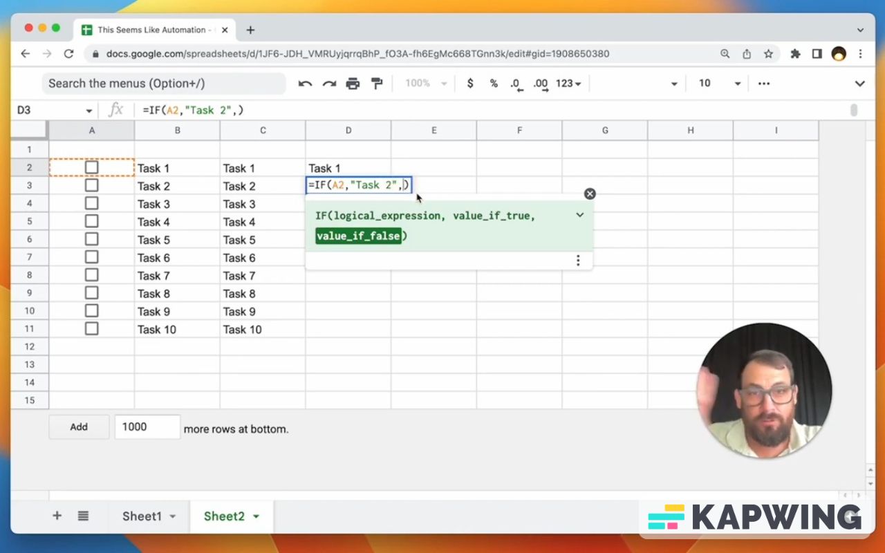
We're going to hit enter. Now when Task 1 is done, check. Task two shows up. So we're going from some nothing to something. We're literally conjuring up here.

We don't have to write in the string here. We can reference something else, like B3. We can do this all the way down. I copied it. There are formulas here, but it looks like there's nothing.

This is a really cool way to really bring some automation in, right? Show the next task when the task is done, or some kind of approval steps. You might be able to do some like fun quizzes in this.

FLATTEN()

This is a little less exciting. BUT SO USEFUL.

Let's create another tab where we have some tasks.

Maybe we're writing down our notes, but they're in many different columns. We have this data that's mangled up.

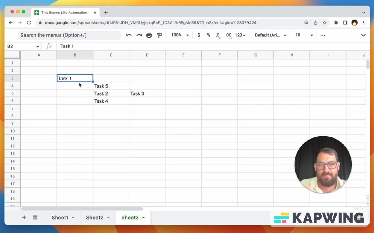
Maybe one of the heartbreaking things is we will use somebody else's data. Somebody else will put something in a sheet and we have to analyze it. We have to manage that data.

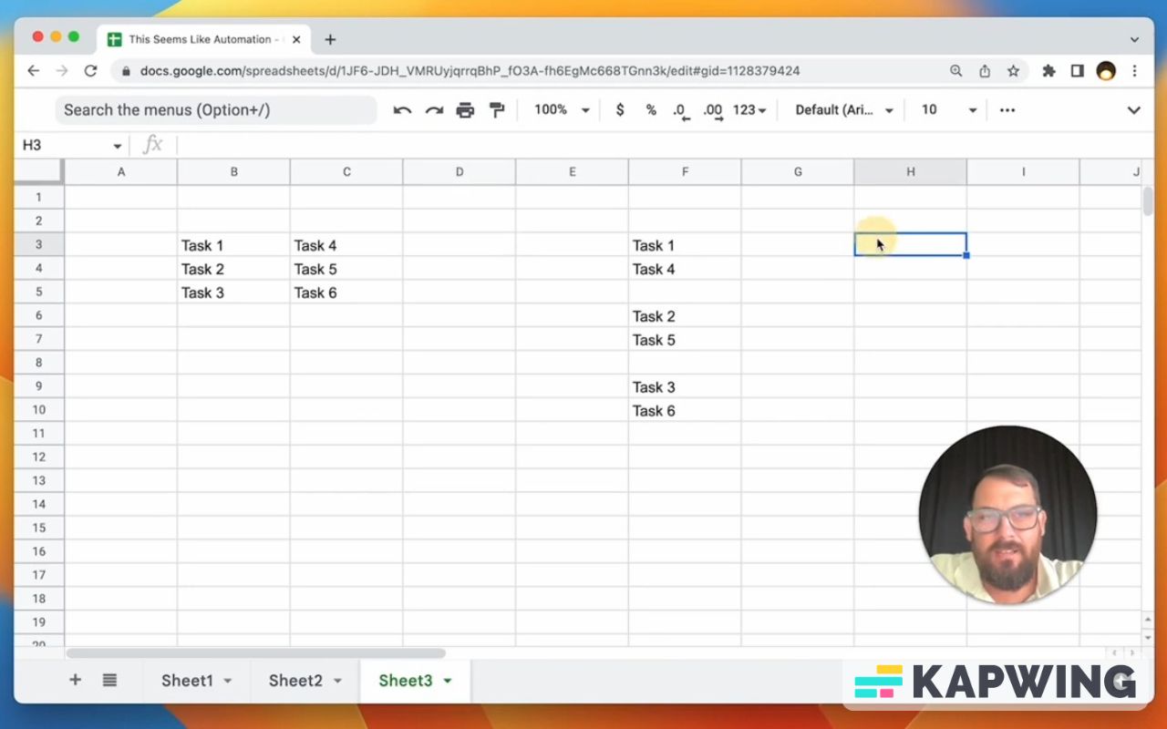
It’s going to take me a while if I list down the tasks again somewhere. What I can do is use FLATTEN(). What this will do is take the whole range and now everything's in one column.

Now there does include the blanks here, because sometimes our data is absolutely full. So you see in our example that Task 1 and Task 4 are horizontal. Each row is getting the column and then it's adding them together all in one column. This is really cool.

You would also want to have something like sort, perhaps.

But this flatten is the key here. Flatten is going to take a wide array of ranges, some columns and rows, and it's going to put it all in one place. This is really cool because we don't have to put Flatten in after the data comes in.

We can put Flatten in a sheet or maybe on another tab and say, “Okay, here's three or four columns.” It’s where you're going to put any information you want here. And then on this other tab, it's going to capture all of that and put it in one column. Very, very useful for certain types of tasks or data entry.

Very, very cool to add Flatten somewhere where the data that's coming in is across many different rows and many different columns specifically.

IFERROR() and FILTER()

The next one is a formula pair if error and filter. Let’s rename Sheet 2 to “IF” and Sheet 3 to “FLATTEN.” Then let’s add another tab, “FILTER.”

You might be familiar with FILTER, but I want to show you one extra thing you can do with IFERROR: We’re going to filter out a column, but we’re going to say only ones in column A and that column B is equal to done. We only want to see the done ones.

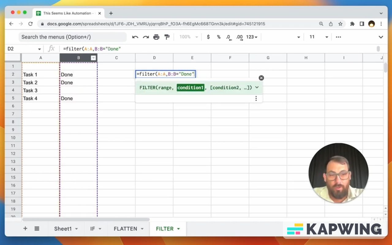
If we get our tasks here, they will automatically show up in this filter. if we have no tasks done, if this filter is empty, we're going to get an error, #N/A, which means no matches are found.

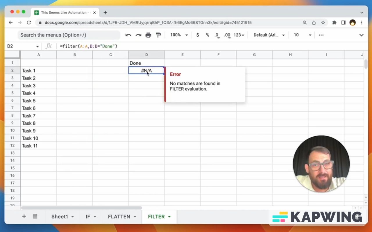
But it's not an error because we're going to fill in something. You can wrap IFERROR. Wrap it around filter and instead of saying “text” here, you can literally do nothing. You can just add that comma, hit enter, and now it's blank. It doesn't show anything until somebody starts typing and done.

Now that's pretty cool, right? It's essentially conjuring a filtered list based on your list that you have here. Like that's really cool. You don't have to show the filter, you don't have to show an error.

I’ll show you one extra thing.

If, however, you do encounter other errors other than #NA and you want to show that. See, if error is going to happen no matter what the error is, but we actually know the actual error is #NA.

So you can do IFNA here. So IFNA is essentially the exact same thing as IF Error, but it will only cover the IFNA error.

And that's really cool because if for some we actually do have a problem with this syntax, it will show up and we'll say, “Okay, we have an error. We have to fix that.”

IFNA is sometimes better if you're not confident about your formula typing and your syntax. I would always recommend. Doing it first without the IF Error or the IFNA. Just do filter alone, get the error, and then put the wrapper on it.

TRANSPOSE() and UNIQUE()

Now, transpose and unique, this is probably one of my funkiest an funniest flavors of formula pairings. It's using transpose, which is a really fun weird sort of weird formula.

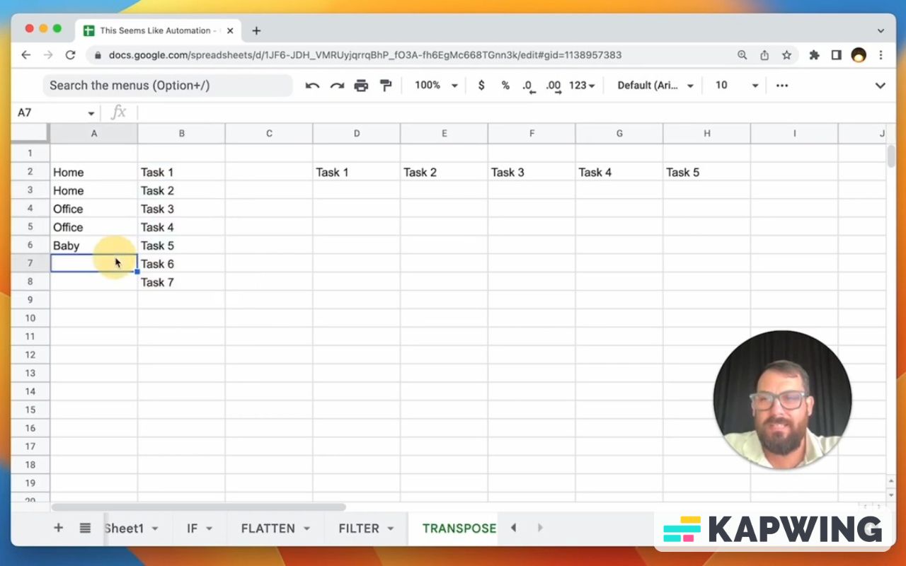
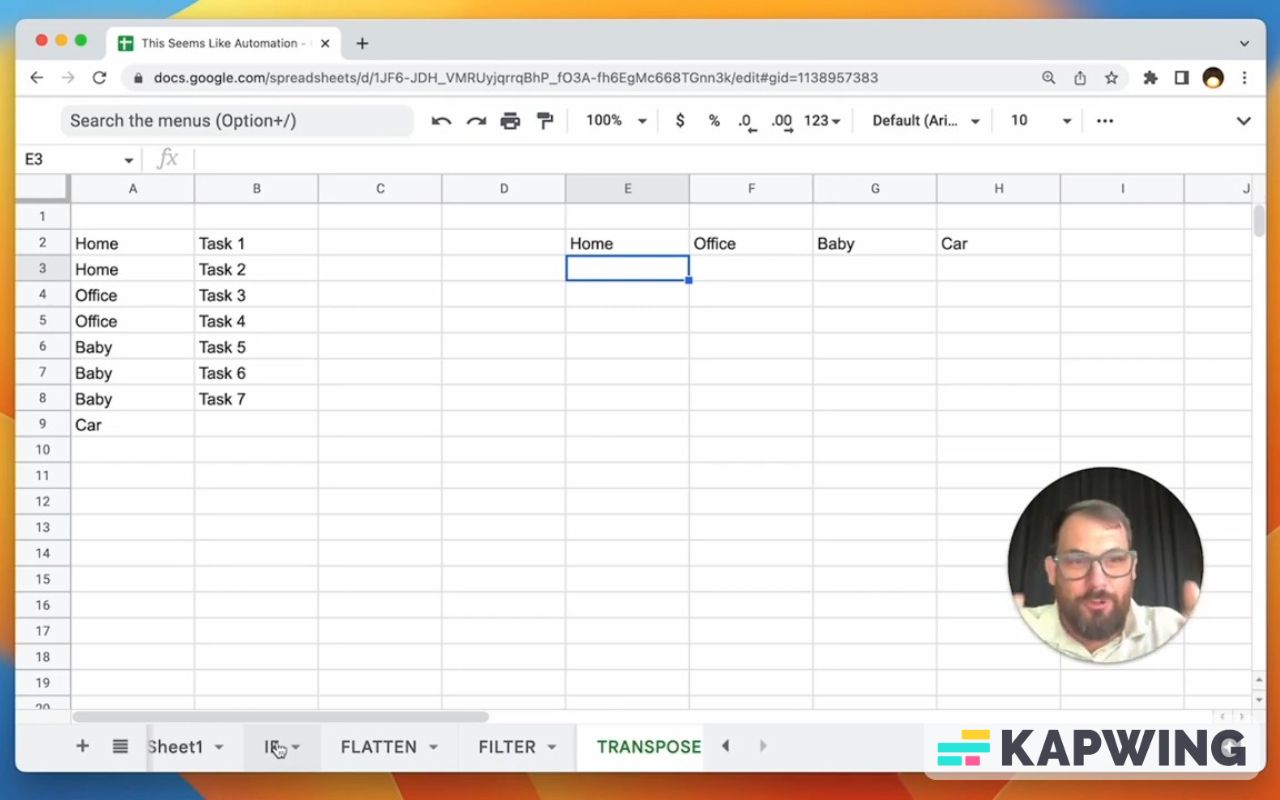
Let's do our task list again. Let’s do =TRANSPOSE and take B2 to B6.

=TRANSPOSE(B2:B6)

What is it? It puts everything horizontal. It literally just changes from a column to a row.

Let’s say we have some categories for these tasks and we want to prioritize the baby stuff.

We have a task list and our categories of what a task is, what this thing we need to do, and we want to create what's like a Kanban board or a Trello board.

I actually have a whole other video about this. Check out Kanban board or Trello board here in Better Sheets.

We'll put a filter here, but what about these headers? What happens if we end up having a different task? We could programmatically or automatically add that to this header list. That's how we use we use Unique and Transpose.

What Unique does is we'll take all the unique of a column. If the car category didn't exist, it would only show home, office, and baby categories. But if we add car, this unique formula is automatically bringing in the car.

This is a list but we want it as headers. So what we can do with our UNIQUE is wrap it with Transpose and let's see what happens there.

Now suddenly, we have all of our headers in exactly the way we want them. Specifically in the order that they are vertically. They will be uniquely our headers.

And all we're doing is taking Transpose and wrapping that around the UNIQUE formula. This is really cool!

If you're a Better Sheets member you will want to check out the actual Kanban board video, go check that out. I have a whole video about using filter and this particular formula pair.

Again, if you’re not confident about Apps Script or you're interested in Apps Script actually automating your sheets: I just released spreadsheet Automation 101. It's available right now on Better sheets.co. If you're a Lifetime member, you have automatic access to it. But also, if you're not a member go check out Spreadsheet Automation 101 on Udemy.

Don’t make any sheets. Make Better Sheets.

Watch the video for this tutorial:

Learn more about automation in Google Sheets:

Get more from Better Sheets

I hope you enjoyed this tutorial! If you want to do more with your Google Sheets, I have other tutorials, like how to create a timer with Apps Script and learning to code with Google Sheets. Beginner? Intermediate? There’s a lot of tutorials for everybody! Check them out at Bettersheets.co.

Join other members. Pay once and own it forever. You get instant access to everything: All the tutorials and templates. All the tools you’ll need. When you’re a member, you get lifetime access to 200+ videos, mini—courses, and Twitter templates. For starters. Find out more here.