Discover Misspelled Duplicates
The built-in feature can sometimes miss duplicates that have subtle differences, such as variations in spacing or formatting. Our formula-based approach, on the other hand, provides a more granular level of control

When working with data in Google Sheets, it's not uncommon to encounter duplicates that are misspelled or have inconsistent formatting. These discrepancies can lead to inaccurate analysis and unreliable results. In this guide, we'll walk you through the process of identifying and correcting these duplicates using powerful formulas like UNIQUE, SORT, COUNTIF, and ARRAYFORMULA. We'll also explore how to handle issues related to capitalization using the LOWER function.
By the end of this tutorial, you'll have the skills to clean up your data, ensure accuracy, and improve the overall quality of your spreadsheets. So, let's dive in and learn how to tame the tangles of duplicate data!
1. Understanding the Problem
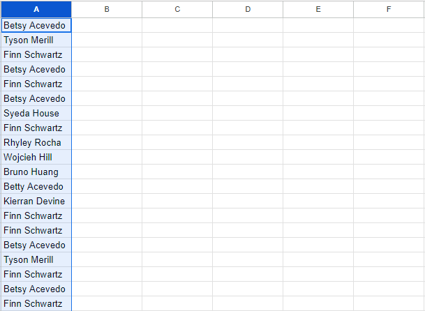
Imagine you're managing a CRM or some other type of database in Google Sheets. Over time, data might be manually entered without proper data validation, leading to inconsistencies. For example:
- "Send" might be entered as "Send," "sended," or even "Send it."
- Names like "Betsy" could appear as "Betty" due to manual entry errors.
Using the built-in "Remove Duplicates" feature in Google Sheets won't help if the duplicates are misspelled or have different capitalizations. Instead, we'll use formulas to detect and fix these issues.
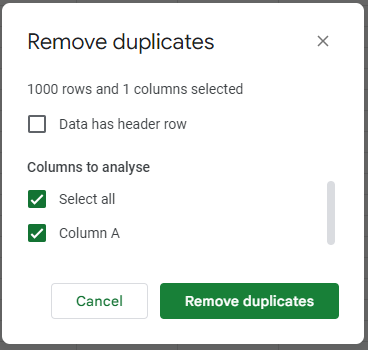
Google Sheets provides a handy tool to help you identify and remove duplicates, to do this:
- Select your data range: Highlight the cells containing the data you want to check for duplicates.
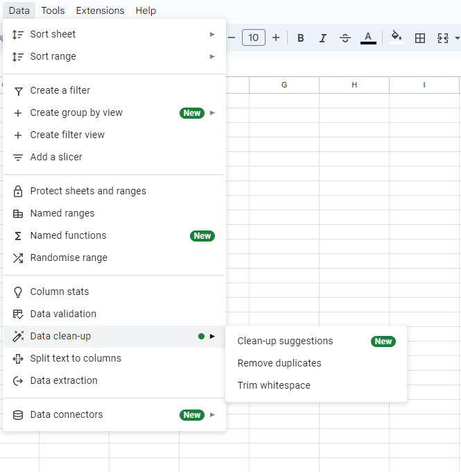
- Access the Data Cleanup tools: Go to the "Data" tab at the top of your Google Sheet.
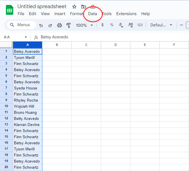
- Choose "Remove duplicates": Click on "Data cleanup" and then select "Remove duplicates."
- Specify columns: If you only want to check for duplicates in specific columns, select the columns you want to include.

- Confirm removal: Click "Remove duplicates" to confirm your action. Google Sheets will remove any rows that contain duplicate values in the selected columns.
2. Identifying Unique Entries
The first step is to identify unique entries in your data. Here's how to do it:
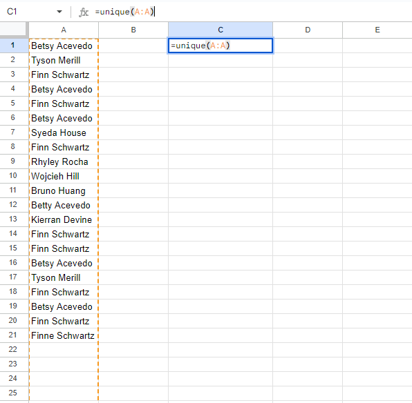
- Use the
UNIQUEFormula: - In a new column, enter the formula
=UNIQUE(A:A), whereA:Arepresents the range of data you want to analyze.
This will create a list of unique entries from the column, but won't eliminate misspelled duplicates.
- Sort the Unique Entries:
- To sort the list alphabetically, wrap the
UNIQUEformula with theSORTfunction:=SORT(UNIQUE(A:A), 1, TRUE).
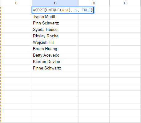
- The
1indicates that you are sorting by the first column, andTRUEsorts the data in ascending order (A to Z).
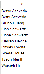
3. Identifying and Correcting Misspelled Duplicates
Once you have a sorted list of unique entries, you can identify and correct duplicates as follows:
- Use the
COUNTIFFormula: - Next to your sorted list, use the
COUNTIFformula to count how many times each entry appears in the original data:=COUNTIF(A:A, C1).
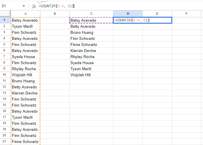
Here, A:A is the range to search, and C1 is the first cell in your sorted list. This will tell you how frequently each entry appears.
- Autofill the Formula:
- After entering the
COUNTIFformula for the first entry, Google Sheets will prompt you to autofill the formula for the rest of the list. Accept the autofill to apply the formula to all entries.
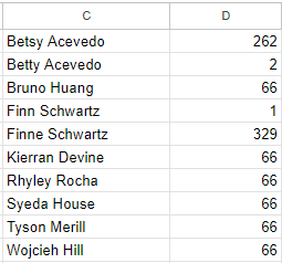
You will immediately see the entries that appear fewer times. For instance, if "Betsy" appears 262 times and "Betty" appears only twice, "Betty" is likely a misspelling of "Betsy."
- Correct the Errors:
- To correct the errors, you can manually find and replace the misspelled entries. Use
Ctrl + F(orCommand + Fon Mac) to search for the misspelled entry and replace it with the correct one.
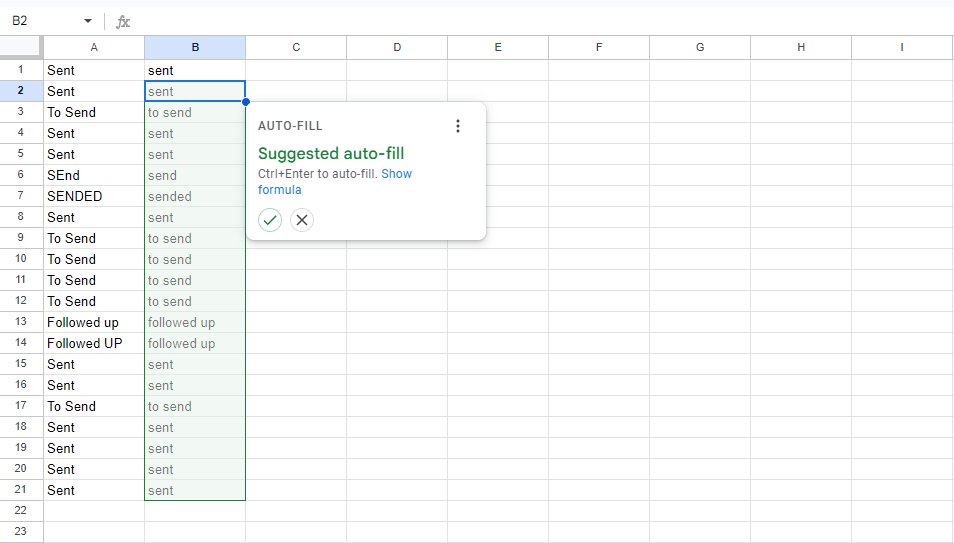
Handling Capitalization Issues
Capitalization differences can also cause issues. For example, "Followed Up" and "followed up" may be treated as different entries. To handle this:
- Convert Text to Lowercase:
- Use the
LOWERfunction to convert all text in a column to lowercase:=LOWER(A1). Autofill the formula down the column to apply it to all entries. To convert text to uppercase, you can use the formula=UPPER(A2). This formula will convert the text in cell A1 to all uppercase letters.
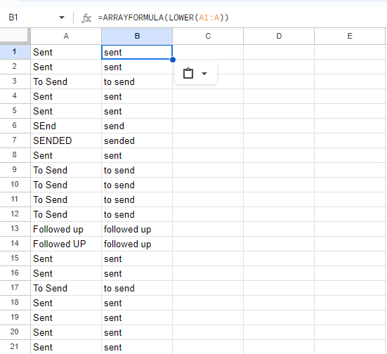
- Use
ARRAYFORMULAfor Bulk Conversion: - Instead of copying the
LOWERfunction down the column, you can useARRAYFORMULAto apply it to the entire range in one step:=ARRAYFORMULA(LOWER(A1:A)). This will automatically convert all entries in column A to lowercase.
By following the steps outlined above, you can effectively clean up your Google Sheets data and ensure that duplicates—whether misspelled or with inconsistent capitalization—are identified and corrected. This method, which leverages formulas like UNIQUE, SORT, COUNTIF, and ARRAYFORMULA, offers a more precise and controlled approach to removing duplicates compared to the built-in "Remove Duplicates" feature.
The built-in feature can sometimes miss duplicates that have subtle differences, such as variations in spacing or formatting. Our formula-based approach, on the other hand, provides a more granular level of control, allowing you to specify exactly how you want to identify and remove duplicates. This ensures that your data remains clean and accurate, setting the stage for reliable analysis and insights.