
Advanced Checkbox Hacks for Streamlined Approvals
Google Sheets is a powerful tool that offers a wide range of functionalities. One such feature that can significantly enhance your workflow is the use of checkboxes for approvals. In this blog post, we will delve into some advanced checkbox hacks in Google Sheets. These tips will help you move beyond simple check marks and emojis, enabling you to create dynamic and flexible approval systems.
Introduction to Checkboxes
Checkboxes in Google Sheets offer a cleaner and more efficient way to handle approvals compared to traditional methods such as emojis or manual check marks. By learning how to use checkboxes effectively, you will streamline processes and be able to manage approvals with ease.
Step-by-Step Guide to Using Checkboxes in Google Sheets
Inserting Checkboxes
First, select an entire column where you want the checkboxes to appear. Then, go to the menu and insert checkboxes. You may notice that the header is altered when you do this, so it's essential to fix your header afterward.
Customizing Checkboxes
Once you've inserted checkboxes, you'll notice that Google Sheets typically labels them as either true or false. To tailor these values to better suit your needs, navigate to "View More Cell Actions" and then go to "Data Validation." Here, you can customize the values to say "Yes" or "No." This modification helps in making the spreadsheet more intuitive and easier to read.
Advanced Usage of Checkboxes
Single Condition Approval
If you need to check multiple columns, but only one approval is required, use the OR function. This enables you to set up a system where any single checkbox being ticked signifies approval.
Here’s a simple formula example:
=OR(B2, C2)
If either B2 or C2 is checked, the condition will be true.
All Conditions Approval
For scenarios requiring all conditions to be met before approval, you will use the AND function. This will check if all specified columns have their checkboxes marked.
Example formula:
=AND(B2, C2)
Both B2 and C2 need to be checked for the condition to be true.
Flexible Approval System
Suppose you need a more flexible system where adding additional approvers doesn’t break your formula. Use the COUNTIF function to adapt to such needs.
For example, if we have four columns B2, C2, D2, and E2, and only one approval is needed, use:
=COUNTIF(B2:E2, TRUE) > 0
This formula will return true if any one of the cells in the range B2 to E2 is checked.
Handling Multiple Approvals
Majority Approval
When your approval system requires a majority vote, modify the COUNTIF function along with logical expressions to handle this.
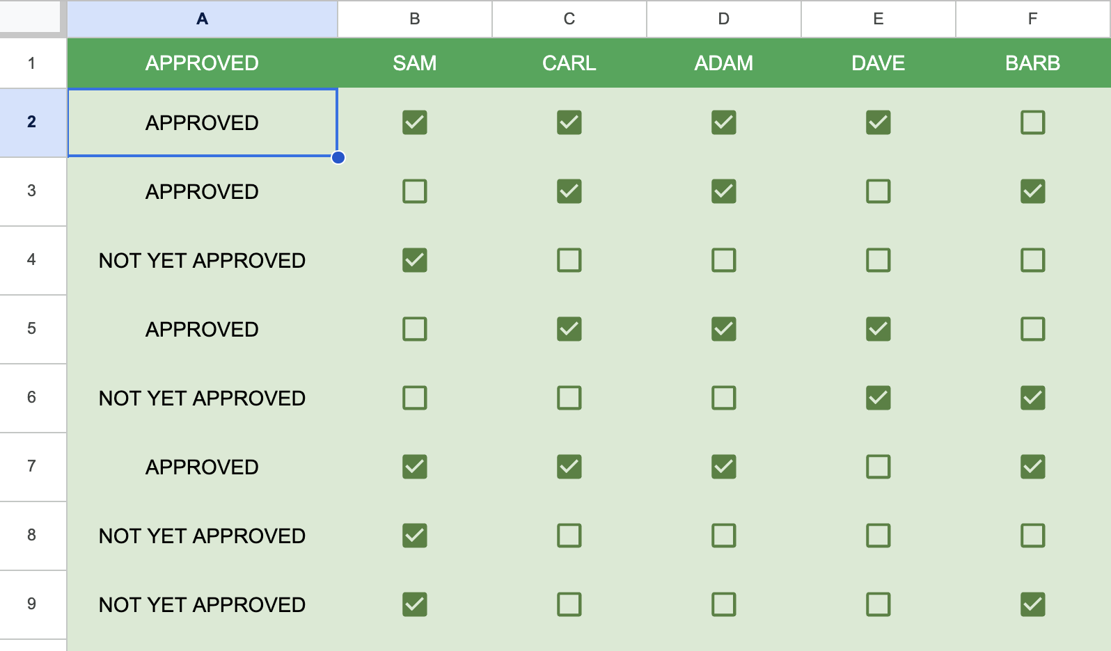
For instance, if there are five potential approvers (columns B2 to F2) and you need at least three approvals to proceed, use:
=COUNTIF(B2:F2, TRUE) >= 3
This formula will ensure that approval is true only if at least three out of the five checkboxes are ticked.
Enhance your efficiency and accuracy
By employing these advanced checkbox hacks, you can significantly enhance your efficiency and accuracy in managing approvals in Google Sheets. Whether you need single approvals, all conditions met, or a majority vote, these methods ensure your approval process is both flexible and foolproof.
We hope these tips have been helpful. Integrating these checkbox techniques into your Google Sheets’ workflow will streamline your approval processes and yield more organized and effective spreadsheets. Happy tweaking!
Watch On YouTube!